【Meachine Learning】05 practical advices
1. feature engineering
2. check model convergence
2.1 how make sure that gradient descent is working well?
- plot the cost function J, which is calculated on the training set.
- This curve is also called a learning curve.
- If J ever increases after one iteration, that means either Alpha is chosen poorly, and it usually means Alpha is too large, or there could be a bug in the code.
2.2 way to decide when your model is done training
- convergence of learning curce
- By 400 iterations, it looks like the curve has flattened out. This means that gradient descent has more or less converged because the curve is no longer decreasing.
- By the way, the number of iterations that gradient descent takes a conversion can vary a lot between different applications.
- automatic convergence test
- threshold epsilon, such as 0.001 or 10^-3.
- If the cost J decreases by less than this number epsilon on one iteration, then you’re likely on this flattened part of the curve that you see on the left and you can declare convergence.
- I usually find that choosing the right threshold epsilon is pretty difficult. I actually tend to look at graphs like this one on the left, rather than rely on automatic convergence tests.
3. about learning rate
multiple learning curve show if learning rate too big.
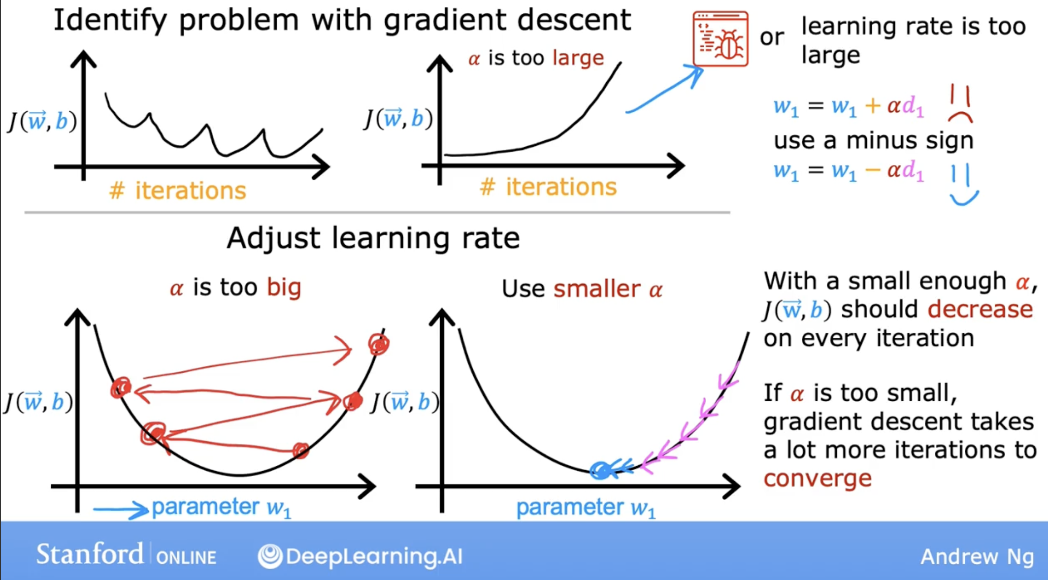
debugging tip:
- with a small enough learning rate.
- if with that, J doesn’t decrease on every single iteration, but instead sometimes increases, then that usually means there’s a bug somewhere in the code.
- and caution is that, this is just a debug method!!!
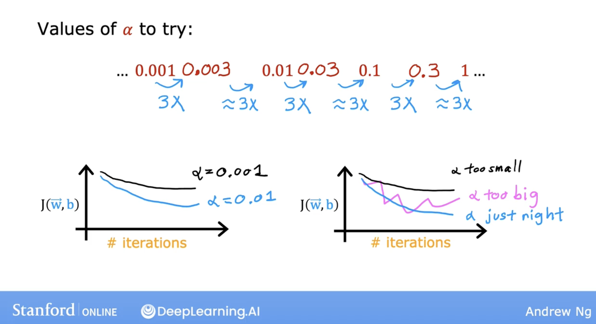
so, how to choose learning rate step:
- 0.001 0.01 1
- 3x
Note: adam optimizer can auto adjust learning rate.
4. underfitting and overfitting
4.1 generalization
Technically we say that you want your learning algorithm to generalize well, which means to make good predictions even on brand new examples that it has never seen before.
4.2 demo of underfitting and overfitting
let’s see some demo:
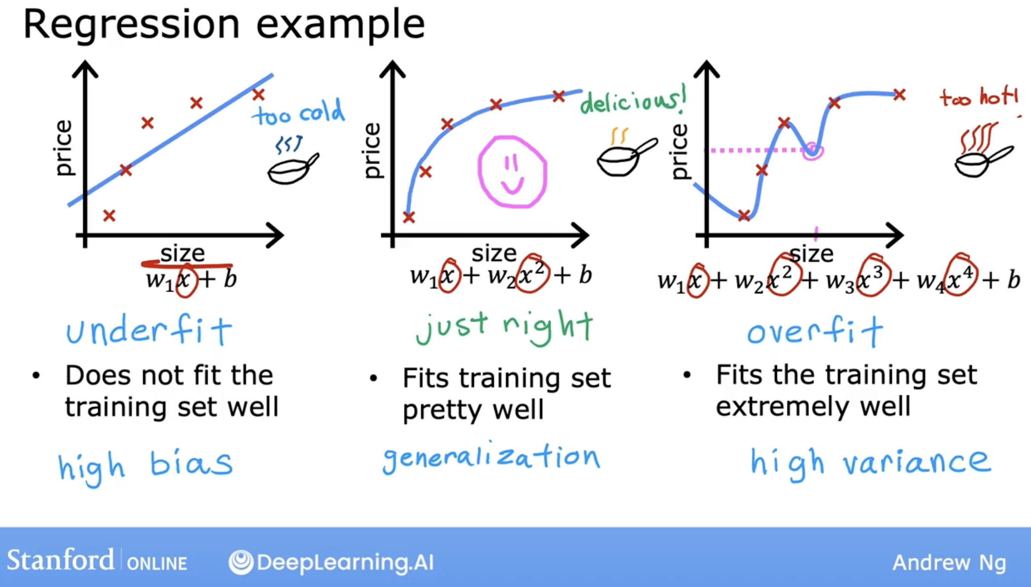
- underfitting and overfitting in linear regression:
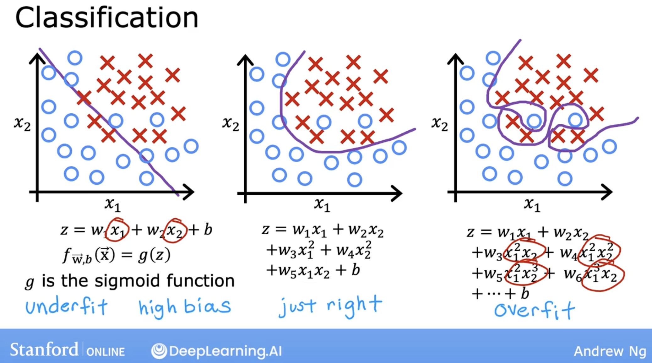
- underfitting and overfitting in logistic regression:
4.3 concept of bias and variance
when underfitting:
- This preconception that the data is linear causes it to fit a straight line that fits the data poorly, leading it to underfitted data.
- this also called
high bias.
when overfitting:
- Because even though it fits the training set very well, it has fit the data almost too well, hence is overfit.
- It does not look like this model will generalize to new examples that’s never seen before.
- this also called
high variance.
4.4 why high variance
The intuition behind overfitting or high-variance is that the algorithm is trying very hard to fit every single training example.
It turns out that if your training set were just even a little bit different, say one house was priced just a little bit more little bit less, then the function that the algorithm fits could end up being totally different.
If two different machine learning engineers were to fit this fourth-order polynomial model, to just slightly different datasets, they couldn’t end up with totally different predictions or highly variable predictions.
That’s why we say the algorithm has high variance.
4.5 how to solve overfitting/high variance?
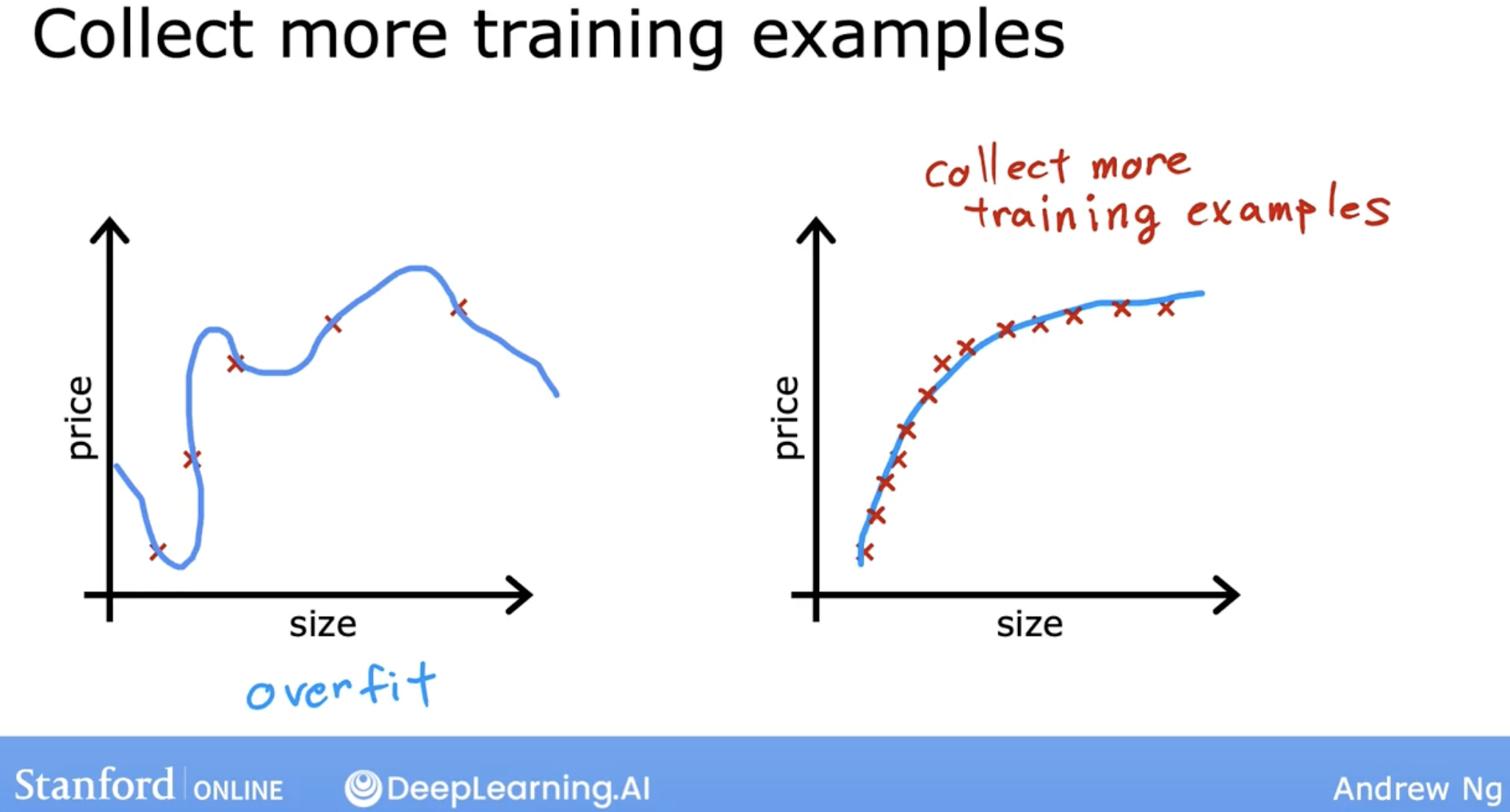
4.5.1 get more training data
4.5.2 feature selection
Here is one feature selection method intuition
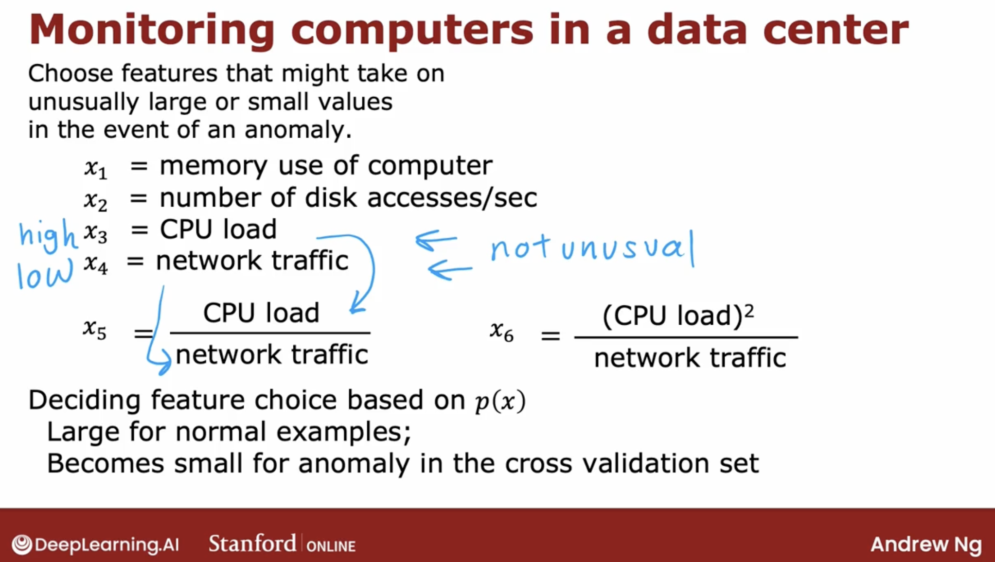
And, feature can be gotten from experience.
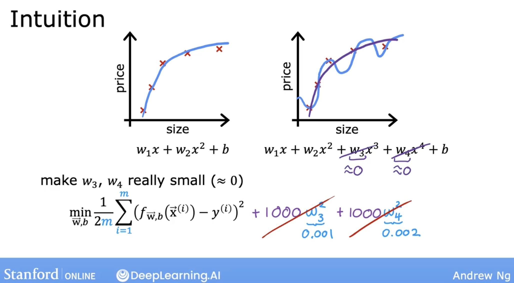
4.5.3 regularization
what is regularization? it looks like we want to penalize the model for having too many large weights with the parameter lambda.
like the following img, we add a parameter lambda to the cost function. the larger the lambda, if we want minimum the cost function, then the weights will be smaller.
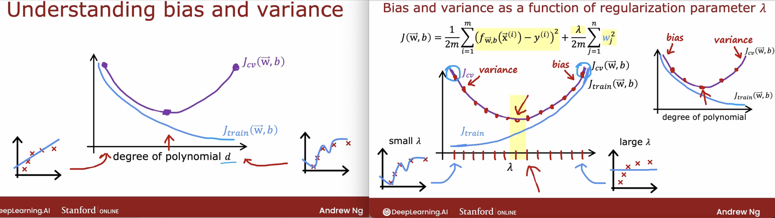
So, when lambda:
- too big: model will underfit;
- too small: model will overfit;
cost function
- linear regression
- without regularization: \(J(w,b) = \frac{1}{2m} \sum\limits_{i = 0}^{m-1} (f_{w,b}(x^{(i)}) - y^{(i)})^2\)
- with regularization: \(J(w,b) = \frac{1}{2m} \sum\limits_{i = 0}^{m-1} (f_{w,b}(x^{(i)}) - y^{(i)})^2 + \frac{\lambda}{2m} \sum\limits_{j=0}^{n-1} w_j^2\)
- logistic regression:
- without regularization: \(J(\mathbf{w}.b) = \frac{1}{m} \sum\limits_{i=0}^{m-1} \left[ (-y^{(i)} \log\left(f_{\mathbf{w},b}\left( \mathbf{x}^{(i)} \right) \right) - \left( 1 - y^{(i)}\right) \log \left( 1 - f_{\mathbf{w},b}\left( \mathbf{x}^{(i)} \right) \right)\right]\)
- with regularization: \(J(\mathbf{w},b) = \frac{1}{m} \sum\limits_{i=0}^{m-1} \left[ -y^{(i)} \log\left(f_{\mathbf{w},b}\left( \mathbf{x}^{(i)} \right) \right) - \left( 1 - y^{(i)}\right) \log \left( 1 - f_{\mathbf{w},b}\left( \mathbf{x}^{(i)} \right) \right) \right] + \frac{\lambda}{2m} \sum\limits_{j=0}^{n-1} w_j^2\)
gradient descent
- linear regression and logistic regression:
- gradient descent approach:
- \[\begin{align*}& \text{repeat until convergence:} \; \lbrace \newline \; & b := b - \alpha \frac{\partial J(\mathbf{w},b)}{\partial b} \newline \; & w_j := w_j - \alpha \frac{\partial J(\mathbf{w},b)}{\partial w_j} \; & \text{for j := 0..n-1}\newline & \rbrace\end{align*}\]
- partial derivatives:
- \[\frac{\partial J(\mathbf{w},b)}{\partial b} = \frac{1}{m} \sum\limits_{i = 0}^{m-1} (f_{\mathbf{w},b}(\mathbf{x}^{(i)}) - \mathbf{y}^{(i)})\]
- \[\frac{\partial J(\mathbf{w},b)}{\partial w_j} = \frac{1}{m} \sum\limits_{i = 0}^{m-1} (f_{\mathbf{w},b}(\mathbf{x}^{(i)}) - \mathbf{y}^{(i)})x_{j}^{(i)} + \frac{\lambda}{m} w_j\]
- gradient descent approach:
- the difference between the two is the $f_{\mathbf{w},b}(\mathbf{x}^{(i)})$
- linear regression: \(f_{\mathbf{w},b}(\mathbf{x}^{(i)}) = \mathbf{w} \cdot \mathbf{x}^{(i)}+b\)
- logistic regression: \(f_{\mathbf{w},b}(\mathbf{x}^{(i)}) = \frac{1}{1+e^{-(\mathbf{w} \cdot \mathbf{x^{(i)}} + b)}}\)
code demo
4.6 how to solve underfitting/high bias?
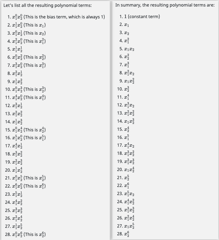
4.6.1 feature mapping
One way to fit the data better is to create more features from each data point. In the provided function map_feature, we will map the features into all polynomial terms of $x_1$ and $x_2$ up to the sixth power.
As a result of this mapping, our vector of two features has been transformed into a 27-dimensional vector.
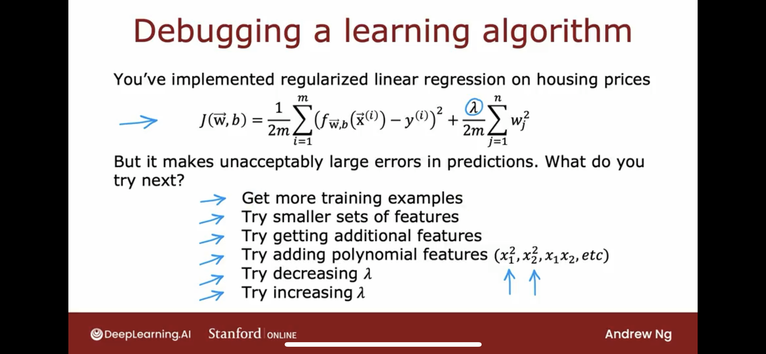
5 decide what to try next
Let’s say you already trained a model, you have the cost, so, how to decide what to do next?
maybe you can have the following chooses
So in order to tell if your model is doing well, especially for applications where you have more than one or two features, which makes it difficult to plot f of x. We need some more systematic way to evaluate how well your model is doing.
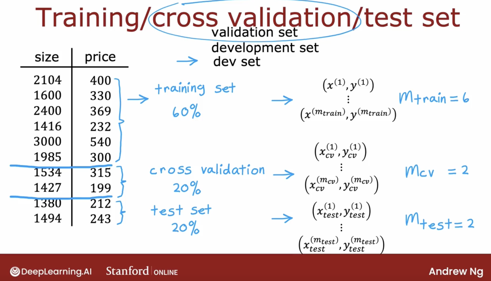
5.1 split the data set to three
The typical workflow of developing a machine learning system is that you have an idea and you train the model, and you almost always find that it doesn’t work as well as you wish yet.
Key to the process of building machine learning system is how to decide what to do next in order to improve his performance.
Because this is a problem with just a single feature x, we could plot the function f and look at it like this. But if you had more features, you can’t plot f and visualize whether it’s doing well as easily.
Instead of trying to look at plots like this, a more systematic way to diagnose or to find out if your algorithm has high bias or high variance will be to look at the performance of your algorithm on the training set and on the cross validation set.
split to three:
| set | rate | usage |
|---|---|---|
| train set | 60% | train the model |
| cross-validation/ validation/ development/ dev set | 20% | use to tune the model |
| test set | 20% | use to evaluate the model |
5.2 the relation of polynomial degree, regularization and bias/variance
5.3 learning curve
What is learning curve? learning curve is a plot of the training and cross validation error as a function of the training set size. like the following.
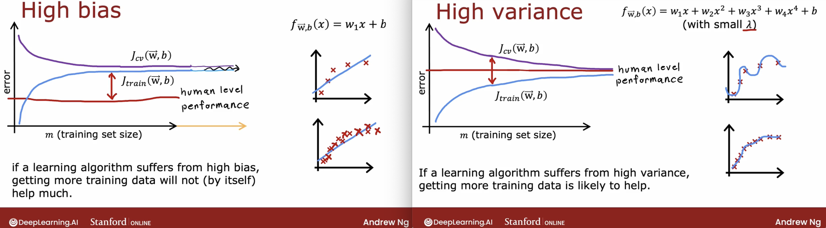
As we can see:
- if the model is high bias, then increase the training set size will not help.
- if the model is high variance, then increase the training set size will help.
5.4 how to evaluate the high bias/high variance?
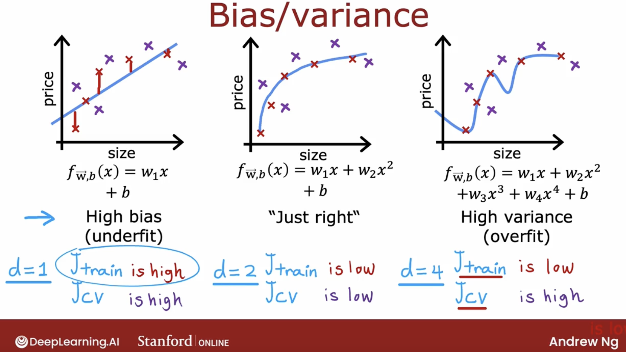
High bias, underfit
- J_train is high
- One characteristic of an algorithm with high bias, something that is under fitting, is that it’s not even doing that well on the training set.
- When J_train is high, that is your strong indicator that this algorithm has high bias.
High variance, overfit
- J_cv is much higher than J_train.
- A characteristic signature or a characteristic Q that your algorithm has high variance will be of J_cv is much higher than J_train.
- In other words, it does much better on data it has seen than on data it has not seen. This turns out to be a strong indicator that your algorithm has high variance.
High bias and high variance at the same time
- The indicator for that will be if the algorithm does poorly on the training set, and it even does much worse than on the training set.
So, there is a question: how to know high? The answer is: baseline.
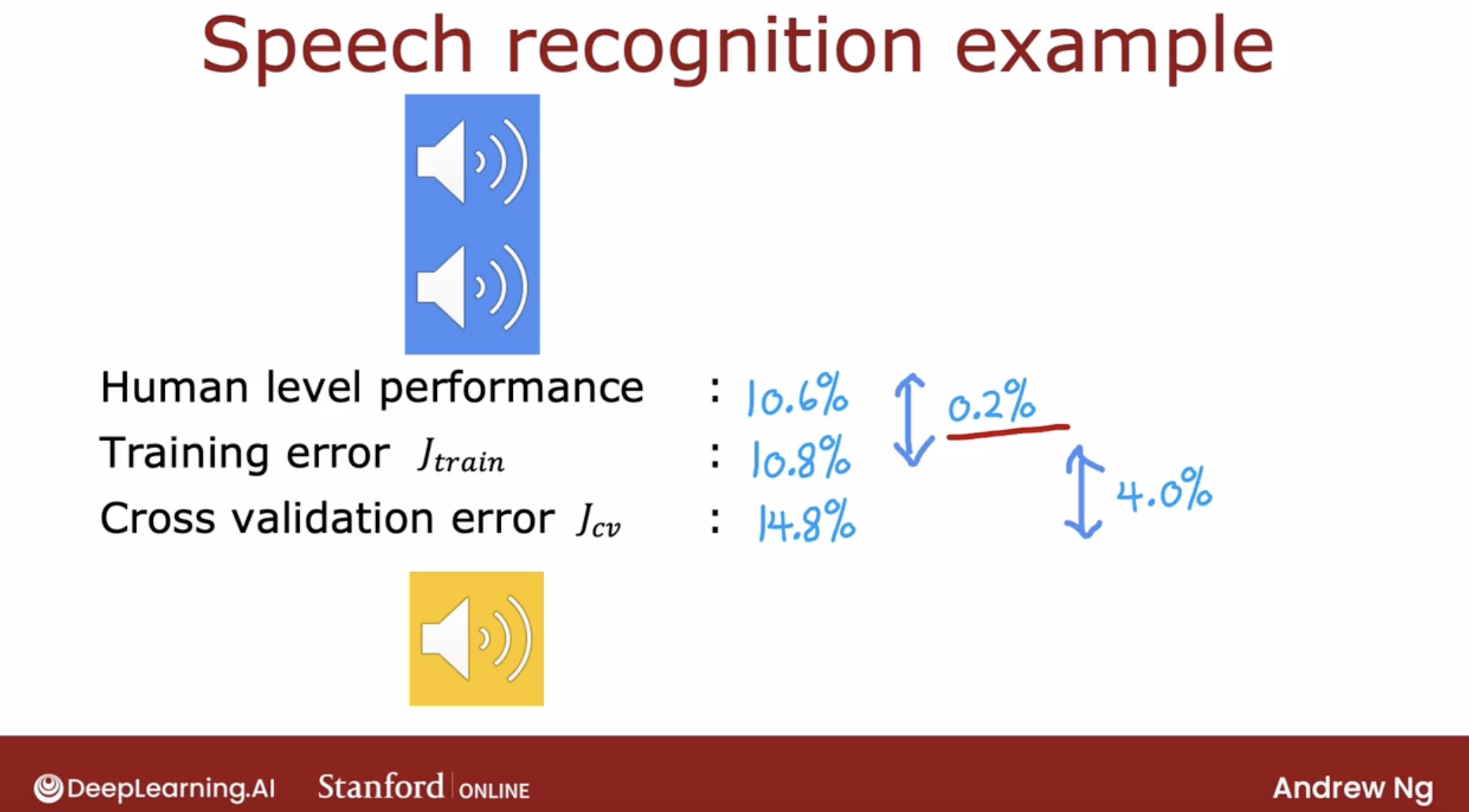
There are three way to get the baseline:
- Human level performance
- Competing algorithm performance
- Guess based on experience
So, with the baseline, we can know whether the algorithm is high bias or high variance.

5.5 summary of what to do
| action | used for |
|---|---|
| Get more training examples | High variance |
| Try smaller sets of features | High variance |
| Try getting additional features | High bias |
| Try adding polynomial features | High bias |
| Try decreasing $\lambda$ | High bias |
| Try increasing $\lambda$ | High variance |
5.6 bias/variance in Neural Networks
But it turns out that neural networks offer us a way out of this dilemma of having to tradeoff bias and variance with some caveats.
And it turns out that large neural networks when trained on small term moderate sized datasets are low bias machines.
And what I mean by that is, if you make your neural network large enough, you can almost always fit your training set well. So long as your training set is not enormous.
So let me share with you a simple recipe that isn’t always applicable. But if it applies can be very powerful for getting an accurate model using a neural network

But I think this recipe explains a lot of the rise of deep learning in the last several years, which is for applications where you do have access to a lot of data. Then being able to train large neural networks allows you to eventually get pretty good performance on a lot of applications.
It turns out that a large neural network with well-chosen regularization, well usually do as well or better than a smaller one.
It hardly ever hurts to have a larger neural network so long as you regularize appropriately. one caveat being that having a larger neural network can slow down your algorithm. So maybe that’s the one way it hurts, but it shouldn’t hurt your algorithm’s performance for the most part and in fact it could even help it significantly.
And second so long as your training set isn’t too large. Then a neural network, especially large neural network is often a low bias machine. It just fits very complicated functions very well, which is why when I’m training neural networks,
I find that I’m often fighting variance problems rather than bias problems, at least if the neural network is large enough. So the rise of deep learning has really changed the way that machine learning practitioners think about bias and variance.
Having said that even when you’re training a neural network measuring bias and variance and using that to guide what you do next is often a very helpful thing to do.
demo of use regularization to control bias and variance
5.7 Error Analysis
5.7.1 what is error analysis?
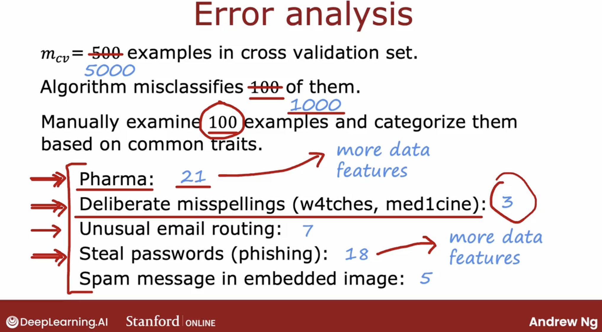
The error analysis process just refers to manually looking through these 100 examples and trying to gain insights into where the algorithm is going wrong.
Specifically, what I will often do is find a set of examples that the algorithm has misclassified examples from the cross validation set and try to group them into common teams or common properties or common traits.
Doesn’t mean it’s not worth doing? But when you’re prioritizing what to do, you might therefore decide not to prioritizes this as highly.
5.7.2 benefit
The point of this error analysis is by manually examining a set of examples that your algorithm is misclassifying or mislabeling. Often this will create inspiration for what might be useful to try next and sometimes it can also tell you that certain types of errors are sufficiently rare that they aren’t worth as much of your time to try to fix.
by error analysis:
- collect more data for specific direction
- add more features for specific direction
- …
5.7.3 limitation
Now one limitation of error analysis is that it’s much easier to do for problems that humans are good at. You can look at the email and say you think is a spam email, why did the algorithm get it wrong?
Error analysis can be a bit harder for tasks that even humans aren’t good at. For example, if you’re trying to predict what ads someone will click on on the website.
But when you apply error analysis to problems that you can it can be extremely helpful for focusing attention on the more promising things to try. That in turn can easily save you months of otherwise fruitless work.
5.7.4 some practical tips
one example can have multiple traits
- Just a couple of notes on this process. These categories can be overlapping or in other words they’re not mutually exclusive.
what to do when cv error examples is too large
- You may not have the time to manually look at all 1,000 examples that the algorithm misclassifies.
- In that case, I will often sample randomly a subset of usually around a 100, maybe a couple 100 examples because that’s the amount that you can look through in a reasonable amount of time.
5.8 skewed-datasets
5.8.1 what is skewed dataset?
what is skewed dataset? why error ratio analysis not effect well?
When working on problems with skewed data sets, we usually use a different error metric rather than just classification error to figure out how well your learning algorithm is doing.
5.8.2 solution of skewed dataset
confusion matrix: precision, recall
- precision: predict right ratio of all predict positive.
- recall: predict right ratio of all actual positive.
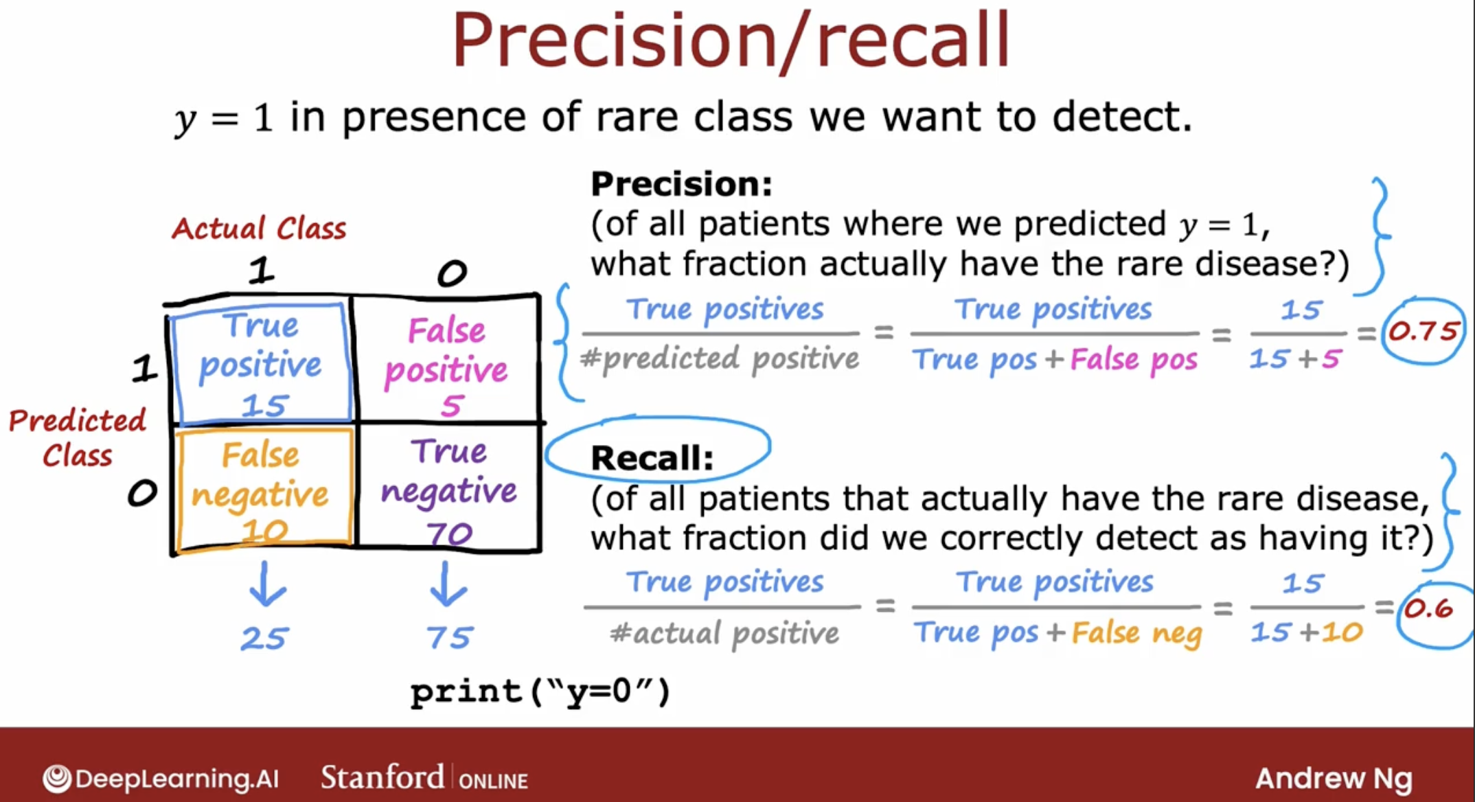
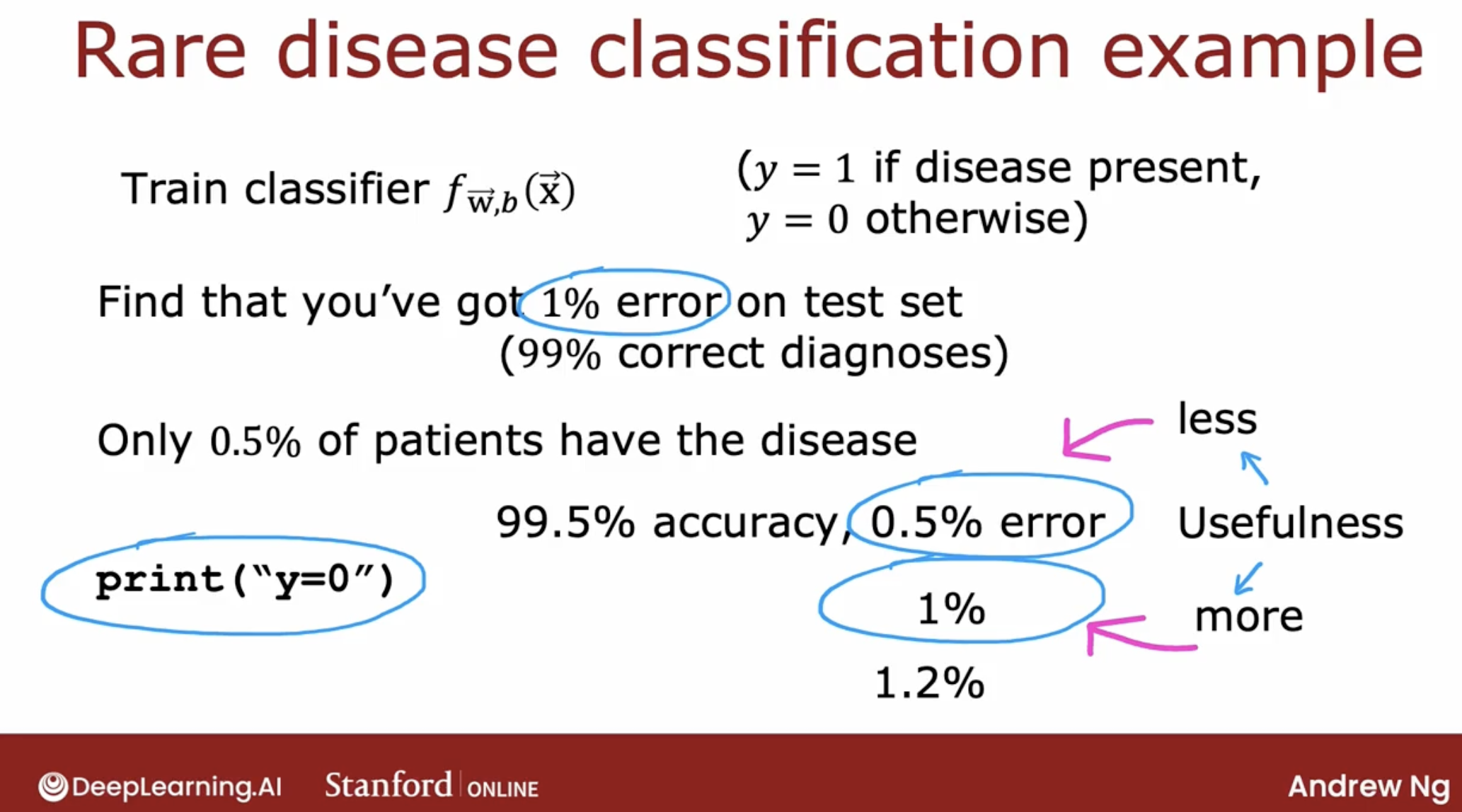
When you have a rare class, looking at precision and recall and making sure that both numbers are decently high, that hopefully helps reassure you that your learning algorithm is actually useful.
5.8.3 trade-off between precision and recall
In the ideal case, we like for learning algorithms that have high precision and high recall.
But it turns out that in practice there’s often a trade-off between precision and recall.
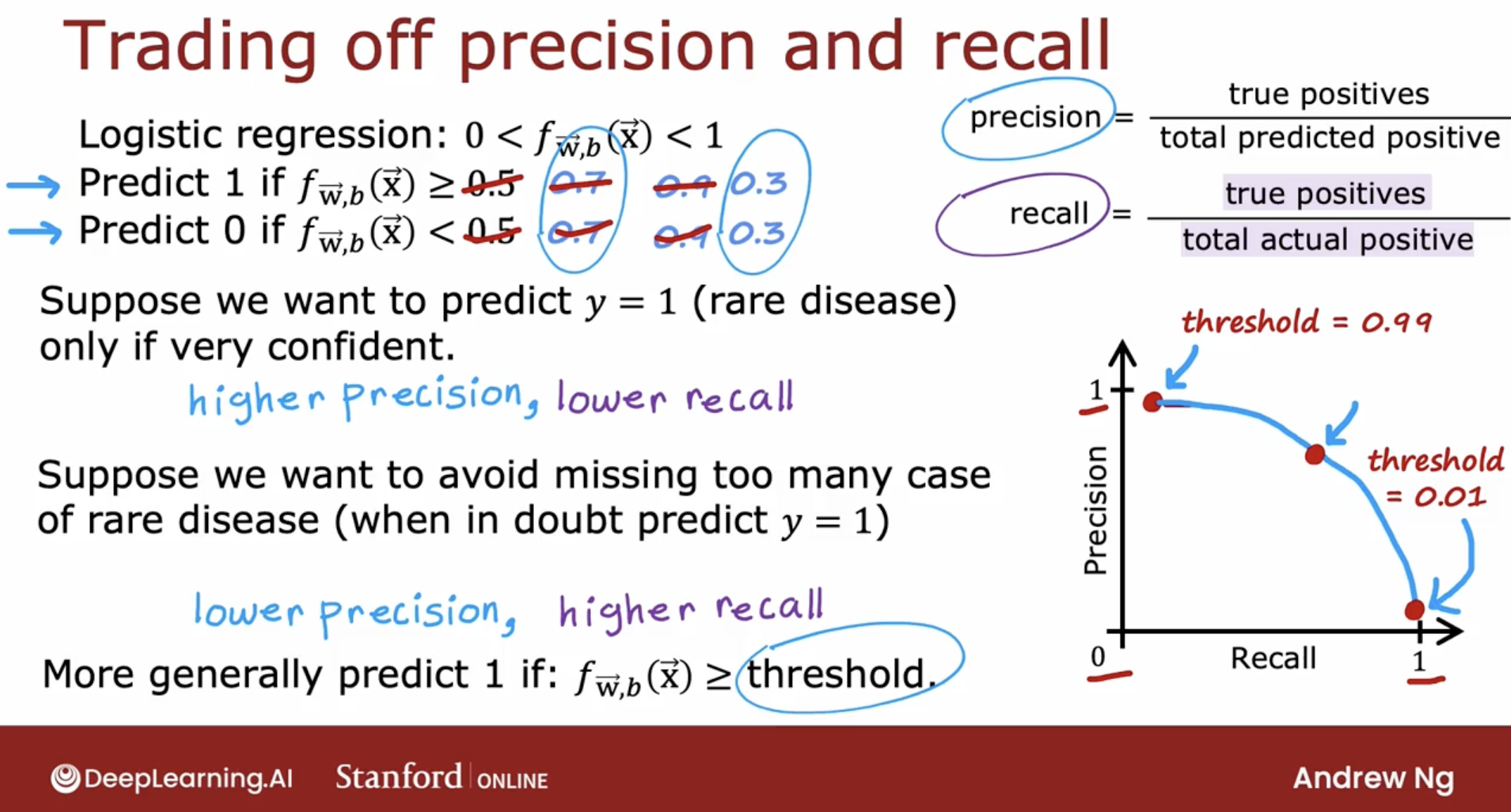
- higher logistic regresstion threshold
If our philosophy is, whenever we predict that the patient has a disease, we may have to send them for possibly invasive and expensive treatment.
If the consequences of the disease aren’t that bad, even if left not treated aggressively, then we may want to predict y equals 1 only if we’re very confident.
In that case, we may choose to set a higher threshold where we will predict y is 1 only if f of x is greater than or equal to 0.7, so this is saying we’ll predict y equals 1 only we’re at least 70 percent sure, rather than just 50 percent sure and so this number also becomes 0.7.
higher threshold, higher precision, lower recall
- lower logistic regresstion threshold
On the flip side, suppose we want to avoid missing too many cases of the rare disease, so if what we want is when in doubt, predict y equals 1, this might be the case where if treatment is not too invasive or painful or expensive but leaving a disease untreated has much worse consequences for the patient.
In that case, you might say, when in doubt in the interests of safety let’s just predict that they have it and consider them for treatment because untreated cases could be quite bad. If for your application, that is the better way to make decisions, then you would take this threshold instead lower it, say, set it to 0.3.
lower threshold, lower precision, higher recall
Notice that picking the threshold is not something you can really do with cross-validation because it’s up to you to specify the best points.
For many applications, manually picking the threshold to trade-off precision and recall will be what you end up doing.
5.8.4 F1 score
But, how to decide the threshold indeed?
In order to help you decide which algorithm to pick, it may be useful to find a way to combine precision and recall into a single score, so you can just look at which algorithm has the highest score and maybe go with that one.
Because it turns out if an algorithm has very low precision or very low recall is pretty not that useful.
F1 Score
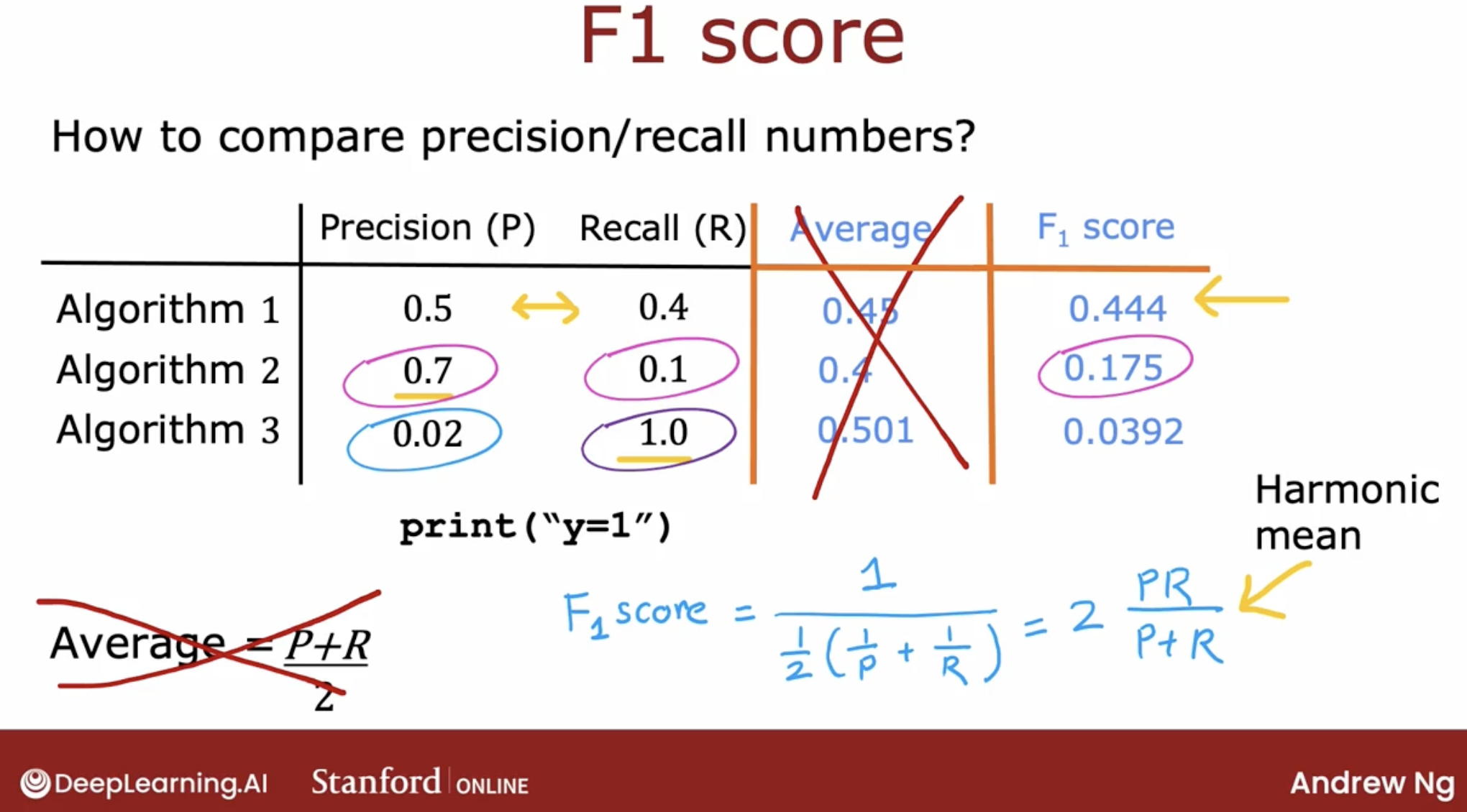
F1 score gives away to trade-off precision and recall, and in this case, it will tell us that maybe the first algorithm is better than the second or the third algorithms.
By the way, in math, this equation is also called the harmonic mean of P and R, and the harmonic mean is a way of taking an average that emphasizes the smaller values more.
6 add data
6.1 how to add data more efficiently
add data for the direction by error analysis
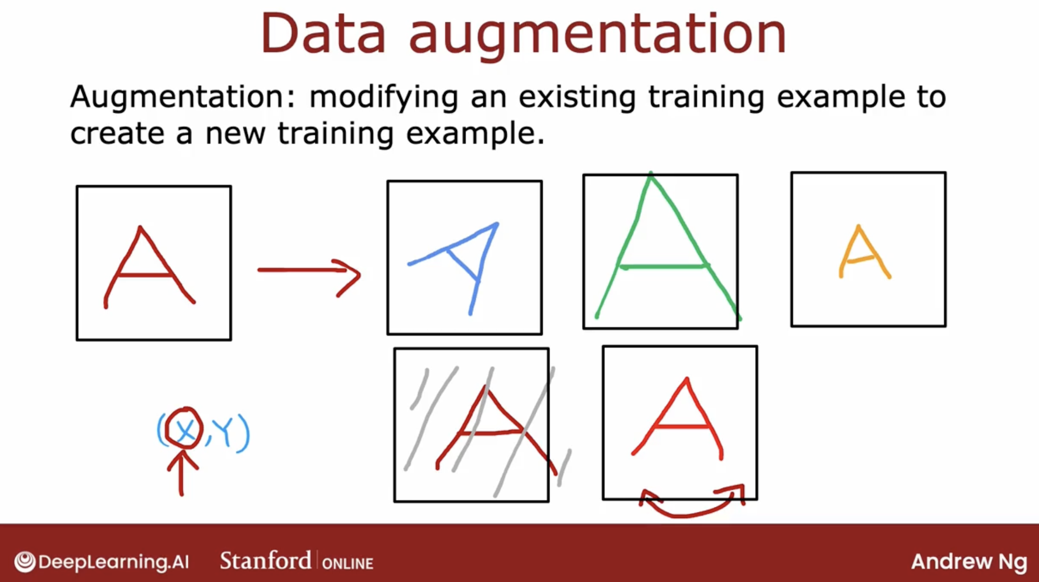
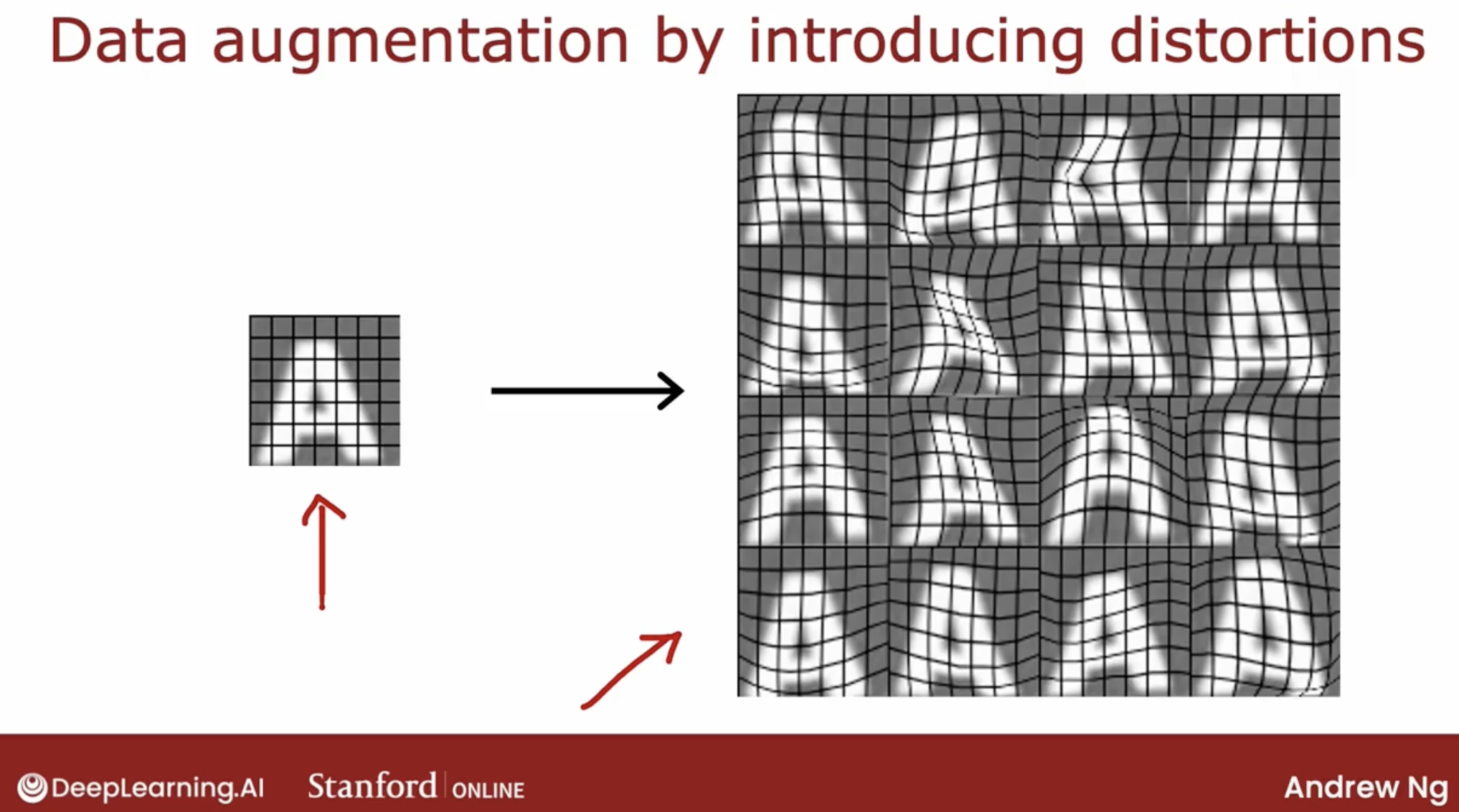
data argument
change or the distort the data
demo:
ocr: image distort, advance add grid upon it
speech: distort the data by add multiple type of noise
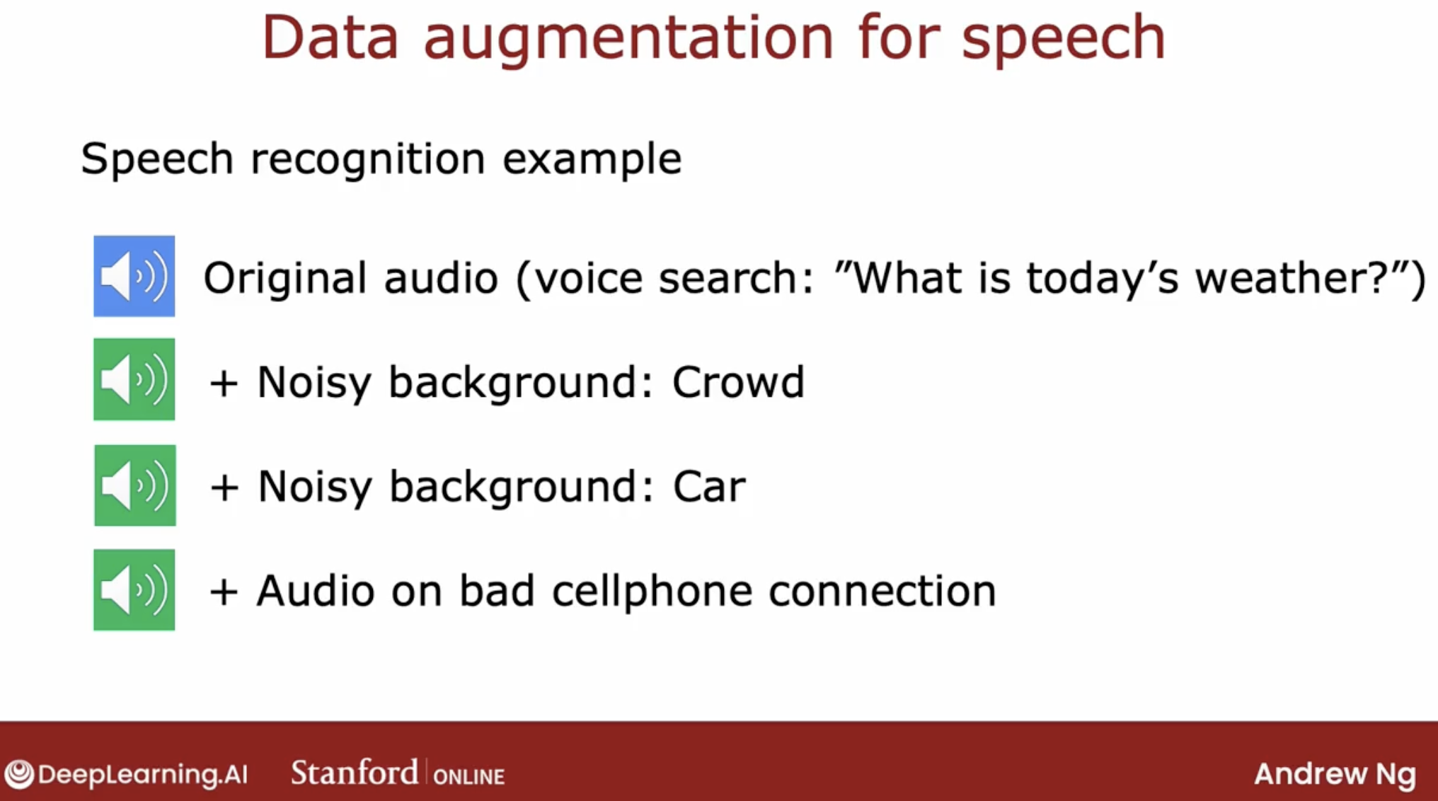
So one way to think about data augmentation is how can you modify or warp or distort or make more noise in your data.
But in a way so that what you get is still quite similar to what you have in your test set, because that’s what the learning algorithm will ultimately end up doing well on.
- data synthesis
demo:
- ocr: generate letter by different font, color, size, angle, shade, etc.
real picture: 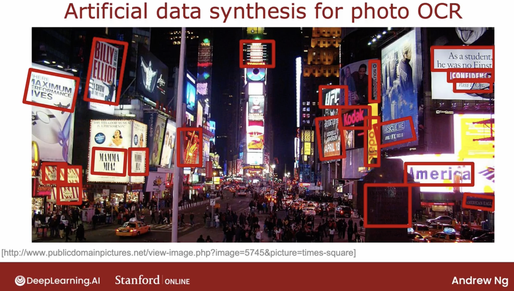
real data from real picture vs synthetic data: 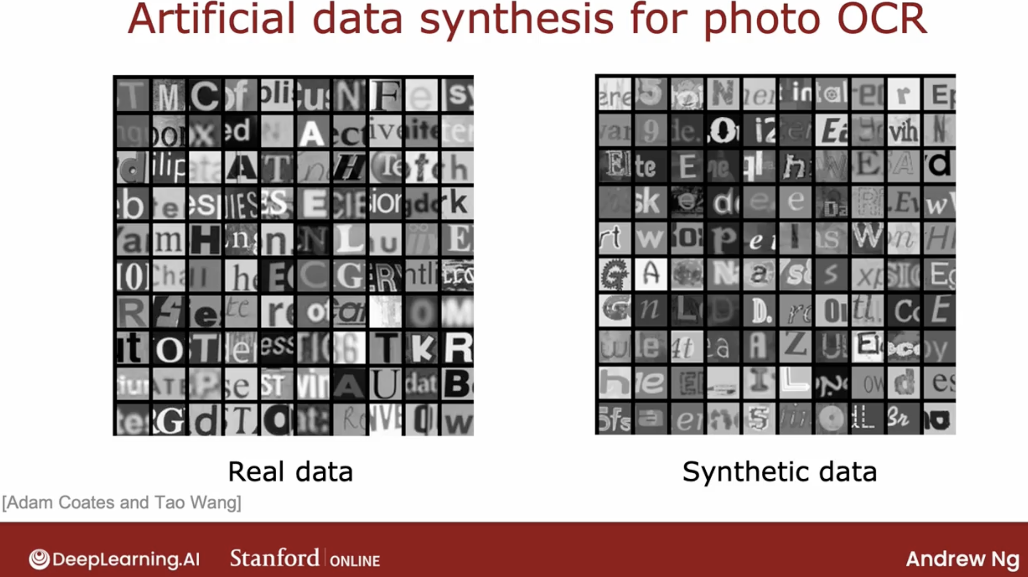
Synthetic data generation has been used most probably for computer vision tasks and less for other applications. Not that much for audio tasks as well.
6.2 work on data is worth
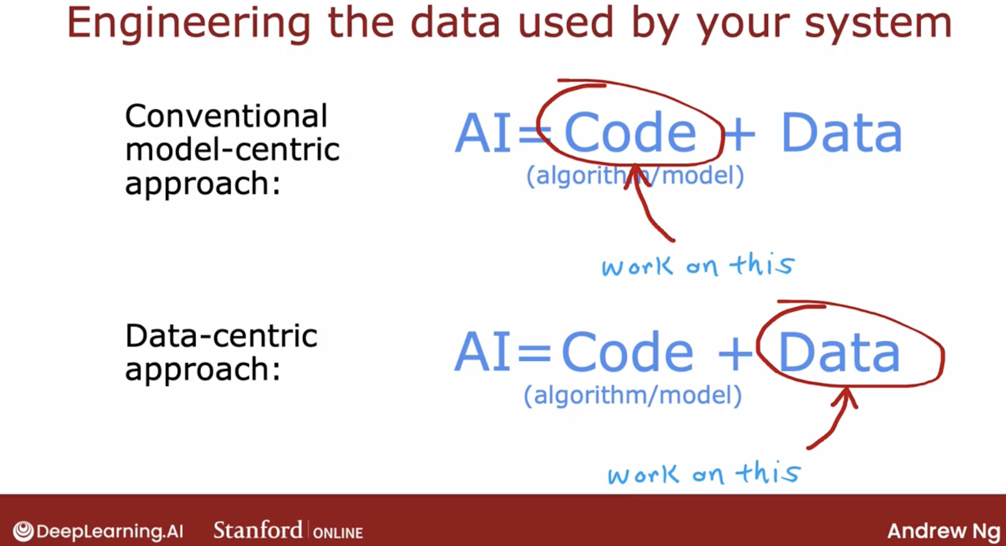
Thanks to that paradigm of machine learning research. I find that today the algorithm we have access to such as linear regression, logistic regression, neural networks, also decision trees we should see next week.
There are algorithms that already very good and will work well for many applications. And so sometimes it can be more fruitful to spend more of your time taking a data centric approach in which you focus on engineering the data used by your algorithm.
And this can be anything from collecting more data just on pharmaceutical spam. If that’s what error analysis told you to do. To using data augmentation to generate more images or more audio or using data synthesis to just create more training examples. And sometimes that focus on the data can be an efficient way to help your learning algorithm improve its performance.
7 iterative loop of train model
iterative-loop: 3 steps
- choose architecture (model, data, feature, lambda, weights, etc)
- train model
- diagnostics (bias, variance, error analysis)
demo: spam filter
- choose architecture:
- choose feature: One way to construct the features of the email would be to say, take the top 10,000 words in the English language or in some other dictionary and use them to define features x_1, x_2 through x_10,000.
- choose weights:
- 0 or 1, depending on whether or not that word appears.
- count the number of times a given word appears in the email.
- choose model:
- Given these features, you can then train a classification algorithm such as a logistic regression model or a neural network to predict y given these features x.
- train model
- diagnositic
- After you’ve trained your initial model, if it doesn’t work as well as you wish, you will quite likely have multiple ideas for improving the learning algorithm’s performance.
- Given all of these and possibly even more ideas, how can you decide which of these ideas are more promising to work on? Because choosing the more promising path forward can speed up your project easily 10 times compared to if you were to somehow choose some of the less promising directions.
- bias and variance
- error analysis
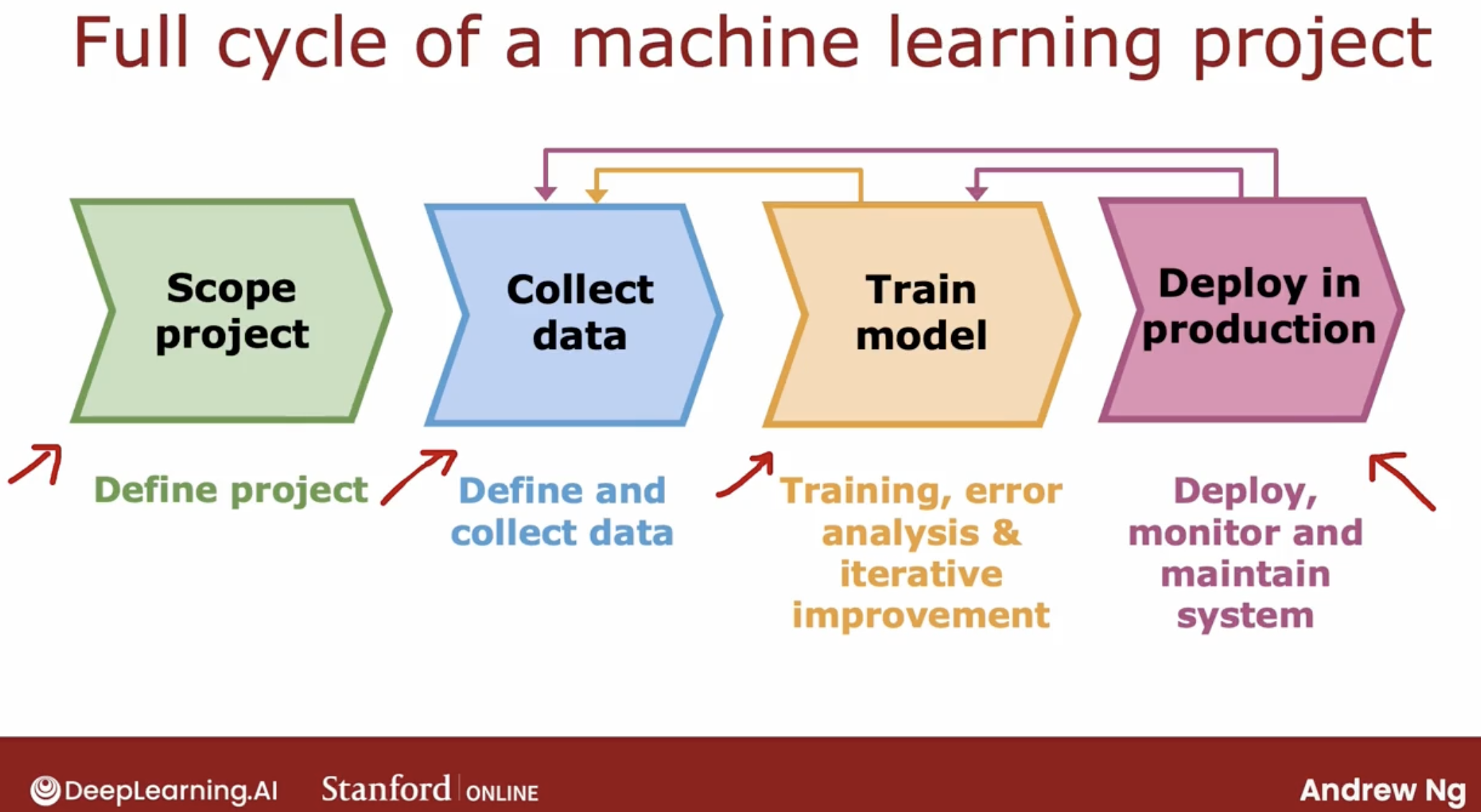
8 full cycle of a machine learning project
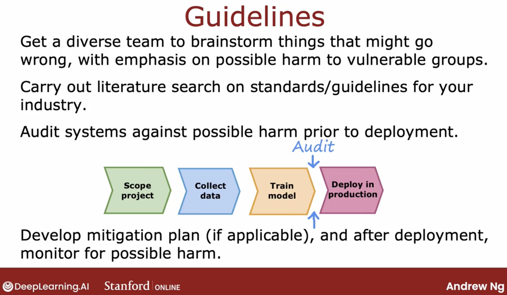
9 ethical considerations
And if you are asked to work on an application that you consider unethical, I urge you to walk away for what it’s worth. There have been multiple times that I have looked at the project that seemed to be financially sound. You’ll make money for some company.
But I have killed the project just on ethical grounds because I think that even though the financial case will sound, I felt that it makes the world worse off and I just don’t ever want to be involved in a project like that.
10 about find optimal hyperparameters
You have demonstrated how to look for the best value hyperparameter-by-hyperparameter. However, you should not overlook that as we experiment with one hyperparameter we always have to fix the others at some default values. This makes us only able to tell how the hyperparameter value changes with respect to those defaults.
In princple, if you have 4 values to try out in each of the 3 hyperparameters being tuned, you should have a total of 4 x 4 x 4 = 64 combinations, however, the way you are doing will only give us 4 + 4 + 4 = 12 results.
To try out all combinations, you can use a sklearn implementation called GridSearchCV, moreover, it has a refit parameter that will automatically refit a model on the best combination so you will not need to program it explicitly.
For more on GridSearchCV, please refer to its documentation.