【Meachine Learning】11 Decision Tree
1 Introduction
1.1 What is Decision Tree?
One of the learning algorithms that is very powerful, widely used in many applications, also used by many to win machine learning competitions is decision trees and tree ensembles.
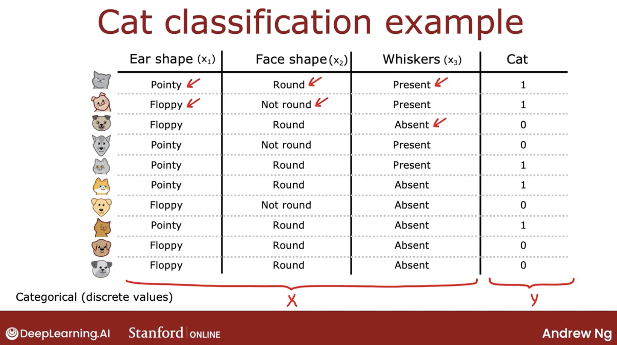
Let’s start with a simple example: cat classification.
key point:
- how to create feature to recognize cat
- MARK: wait to complete.
1.2 Notation
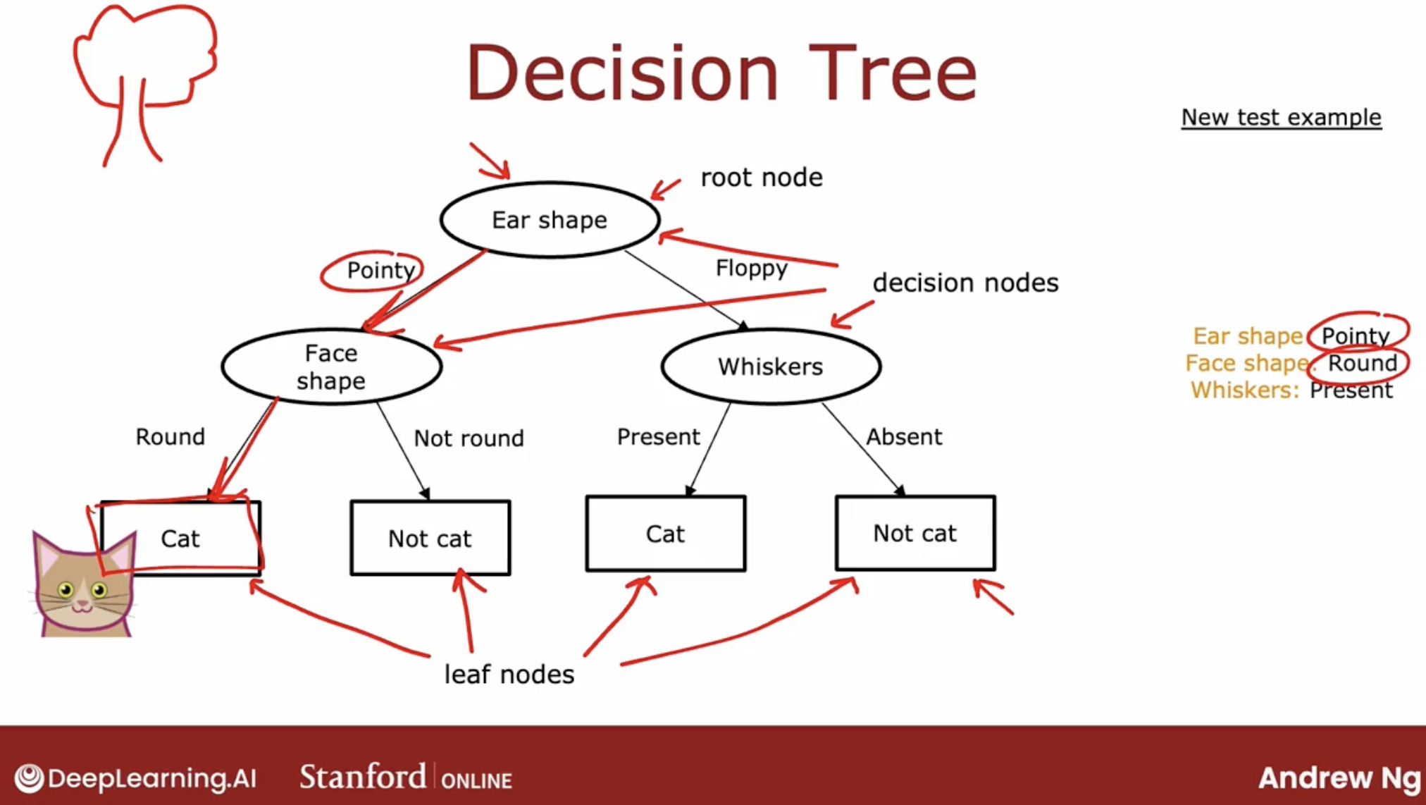
decision tree notation
- root node
- decision nodes
- leaf nodes
one example of decision tree
So, the job of the decision tree learning algorithm is:
- out of all possible decision trees, to try to pick one that hopefully does well on the training set
- and then also ideally generalizes well to new data such as your cross-validation and test sets as well.
Seems like there are lots of different decision trees one could build for a given application.
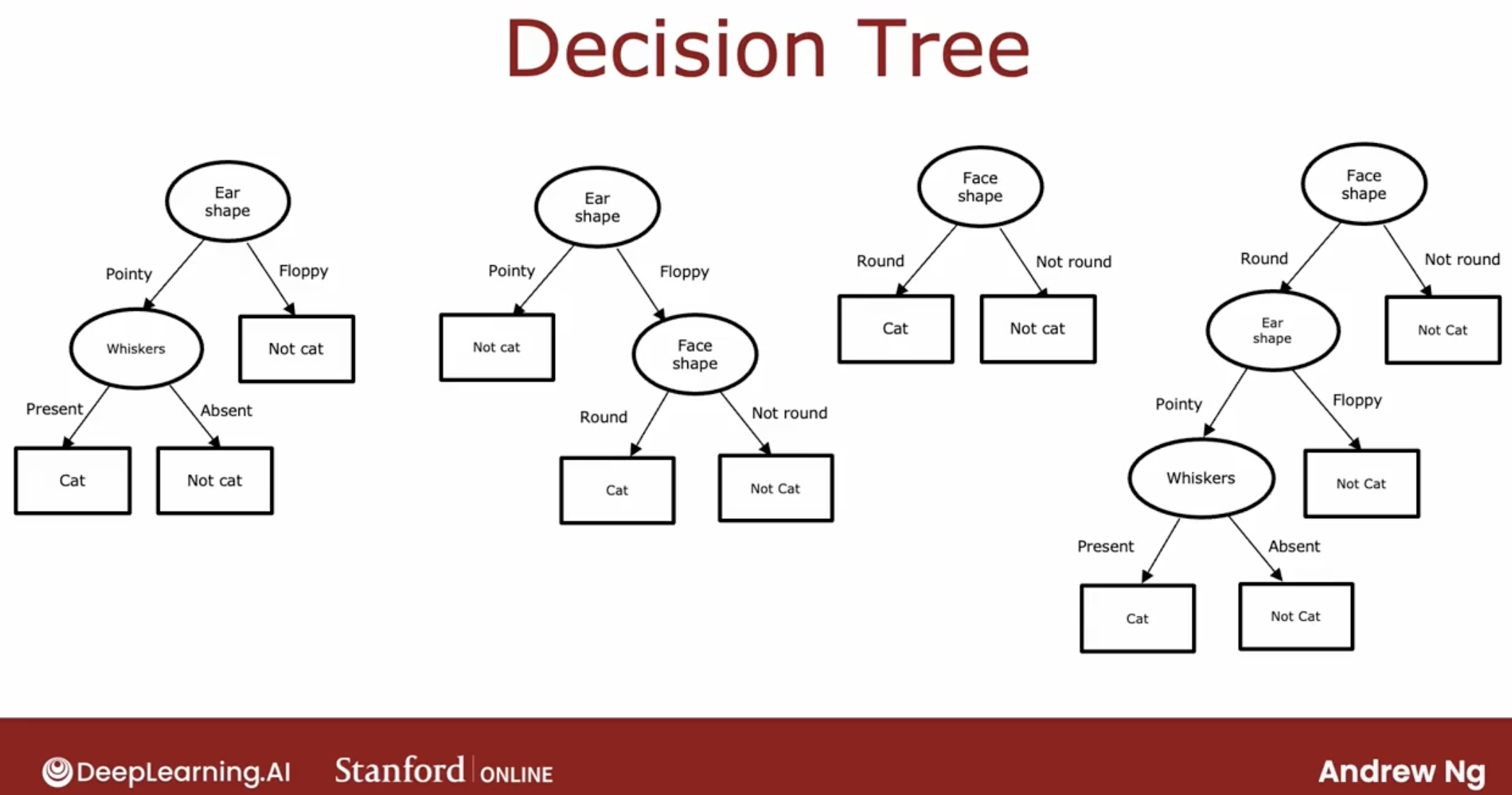
How do you get an algorithm to learn a specific decision tree based on a training set?
2 Two question of decision tree learning algorithm
The process of building a decision tree given a training set has a few steps.
- decide what feature to use at the root node.
- iterate get all decision nodes, until get leaf nodes
So, here is the two decision of decision tree learning algorithm:
- how to choose what features to use to split on at each node?
- how to choose what values to split on at each node?
2.1 maximize purity
how do you choose what features to use to split on at each node?
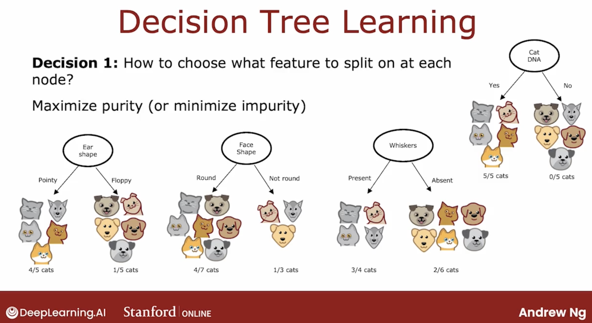
Answer is maximize purity. By purity, I mean, with the features that we actually have, you want to get to what subsets, which are as close as possible to all cats or all dogs.
Because it is if you can get to a highly pure subsets of examples, then you can either predict cat or predict not cat and get it mostly right.
But how to get to a highly pure subset? we will see later.
2.2 stop splitting
when do you stop splitting?
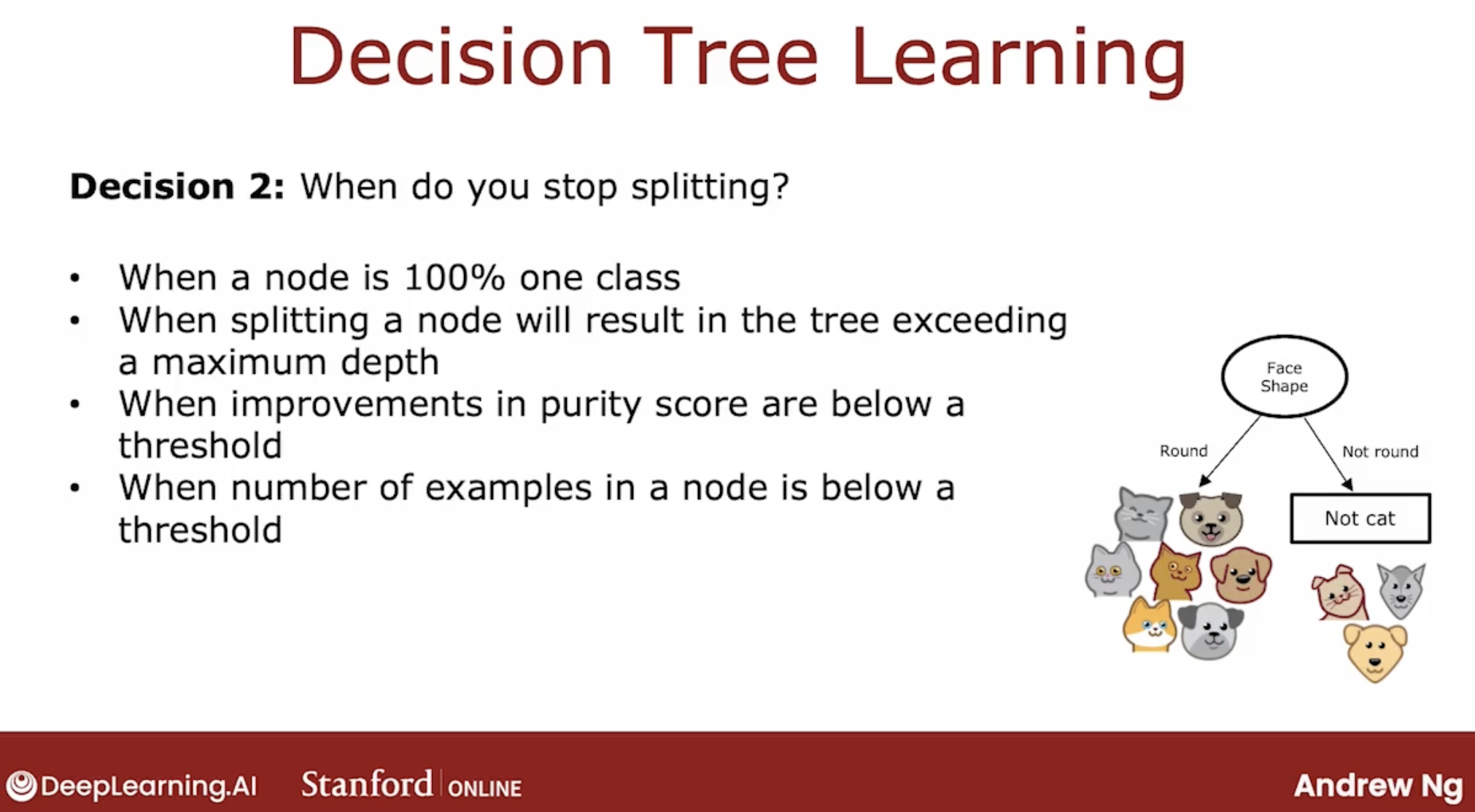
In decision tree, the depth of a node is defined as the number of hops. root node is depth 0.
why limit the depth:
- tree don’t get too big and unwieldy
- less prone to to overfit
Over the years, different researchers came up with different refinements to the algorithm.
As a result of that, it does work really well but we look at all the details of how to implement a decision tree. It feels a lot of different pieces such as why there’s so many different ways to decide when to stop splitting.
If it feels like a somewhat complicated, messy algorithm to you, it does to me too. But these different pieces, they do fit together into a very effective learning algorithm and what you learn in this course is the key, most important ideas for how to make it work well.
3 Choose feature to split
3.1 Entropy
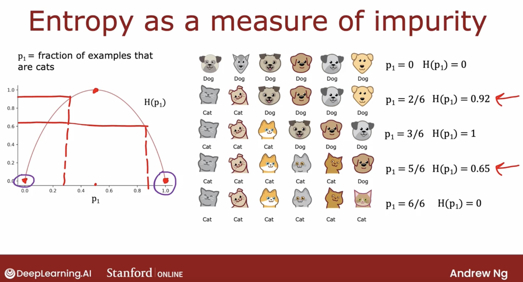
But, what does it mean to be highly pure? Let’s have a look at entropy.
What’s entropy?
what’s the formula?
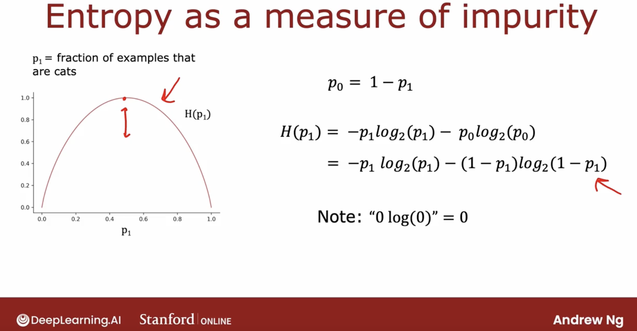
why log_2:
- we have 2 categories
- use 2 can let the peak of the curve equal to 1
To summarize, the entropy function is a measure of the impurity of a set of data. It starts from zero, goes up to one, and then comes back down to zero as a function of the fraction of positive examples in your sample.
There are other functions that look like this, they go from zero up to one and then back down. For example, Gini criteria.
3.2 Information gain
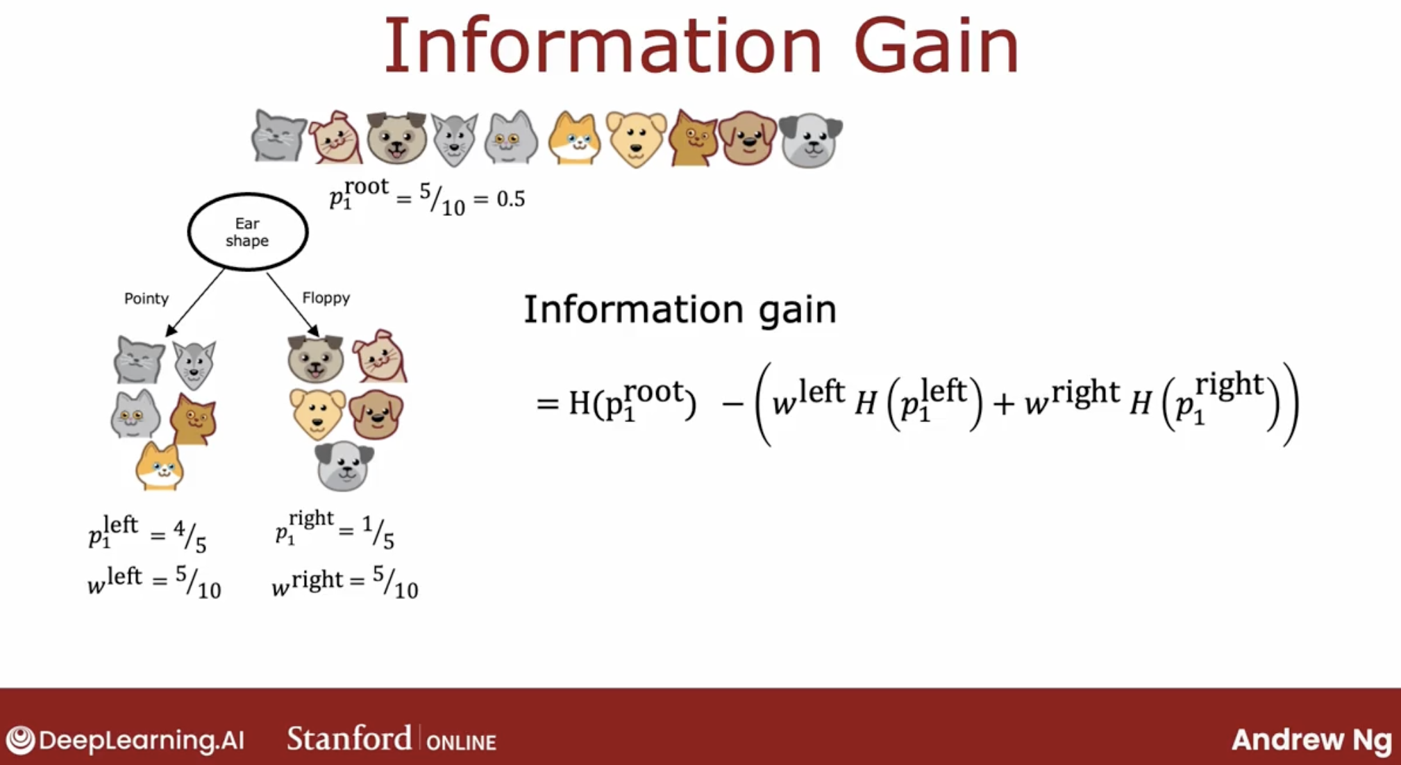
When building a decision tree, the way we’ll decide what feature to split on at a node will be based on what choice of feature reduces entropy the most. Reduces entropy or reduces impurity, or maximizes purity.
In decision tree learning, the reduction of entropy is called information gain.
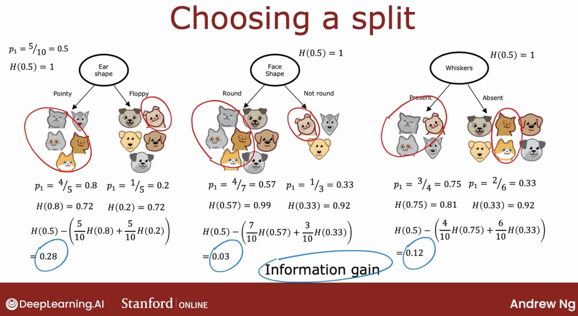
So you can just pick of these three choices, which one does best? The way we’re going to combine these two numbers is by taking a weighted average.
Why do we bother to compute reduction in entropy rather than just entropy at the left and right sub-branches? It turns out that one of the stopping criteria for deciding when to not bother to split any further is if the reduction in entropy is too small.
And here is the notation for the information gain.
3.3 summary
So, here is the summary of Decision Tree Learning Algorithm:
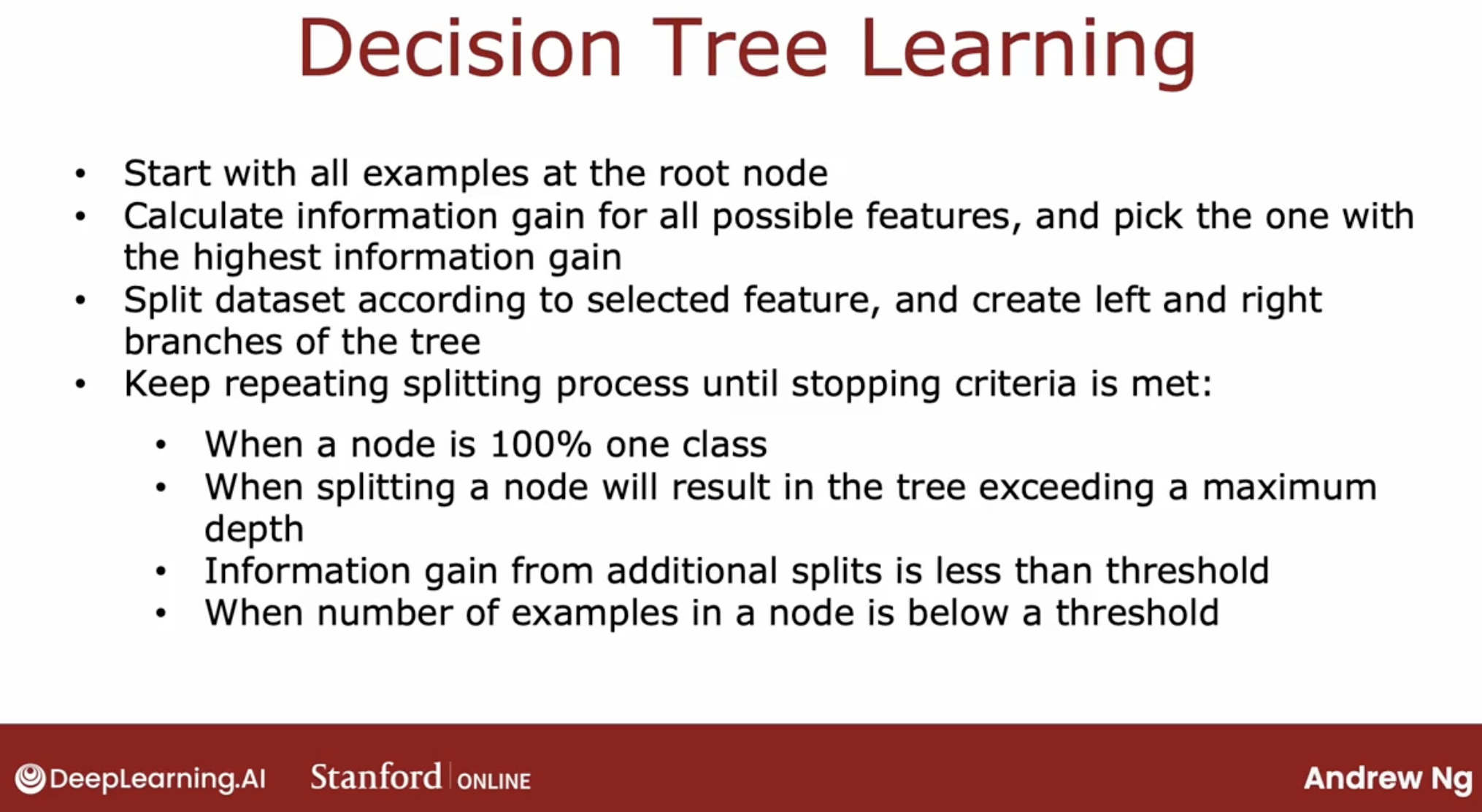
this will use recursive algorithm.
In theory, you could use cross-validation to pick parameters like the maximum depth, where you try out different values of the maximum depth and pick what works best on the cross-validation set. Although in practice, the open-source libraries have even somewhat better ways to choose this parameter for you.
other condition or criteria, open-source libraries are provide also.
4 handle feature
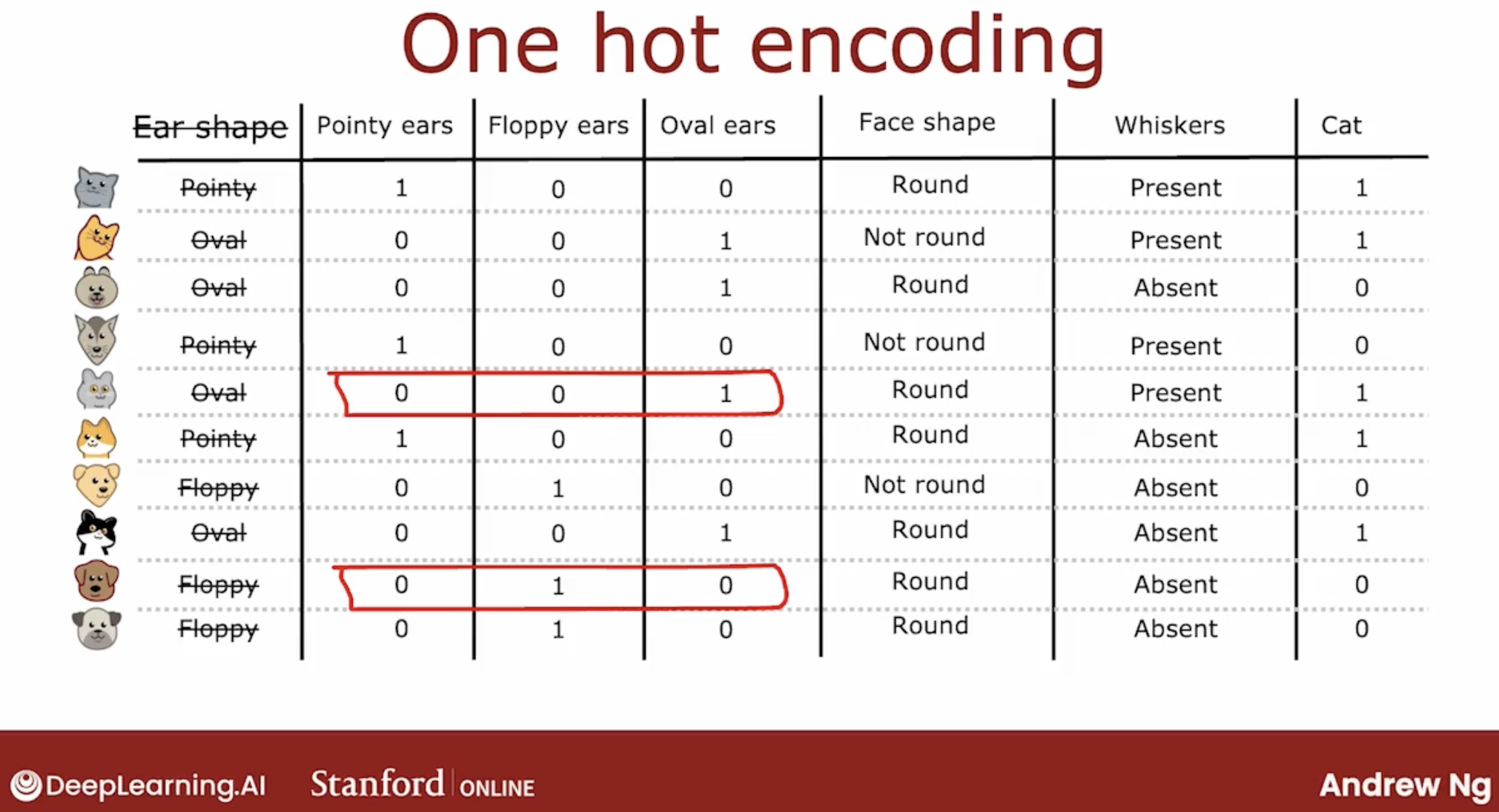
4.1 one-hot encoding
In a little bit more detail, if a categorical feature can take on k possible values, k was three in our example, then we will replace it by creating k binary features that can only take on the values 0 or 1.
Just an aside, even though this week’s material has been focused on training decision tree models, the idea of using one-hot encodings to encode categorical features also works for training neural networks.
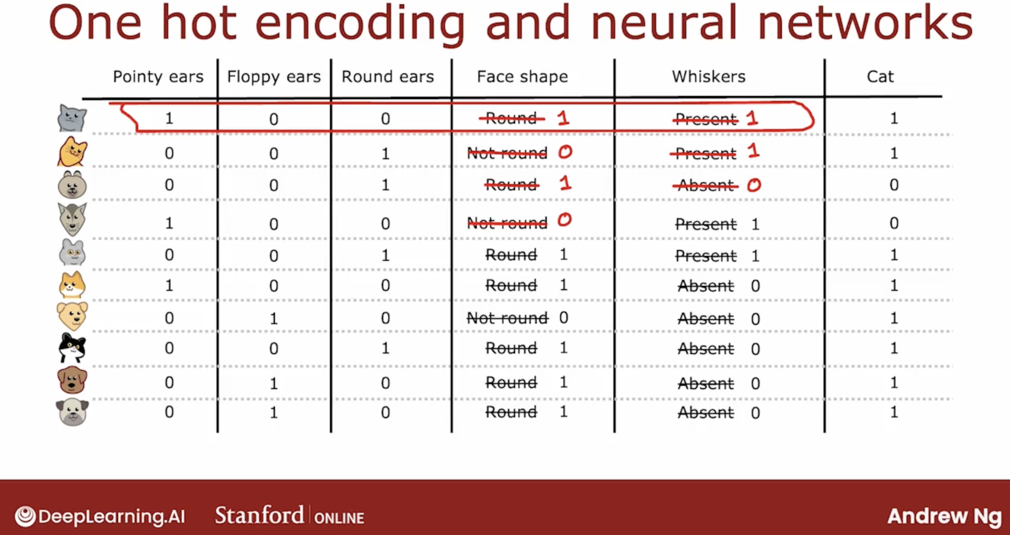
So one-hot encoding is a technique that works not just for decision tree learning but also lets you encode categorical features using ones and zeros, so that it can be fed as inputs to a neural network or a linear regression or a logistic regression as well which expects numbers as inputs.
4.2 splitting on continuous features
Let’s look at how you can modify decision tree to work with features that aren’t just discrete values but continuous values.
Also split this feature by the best way.
And what we should do when constraints splitting on the weight feature is to consider many different values of this threshold and then to pick the one that is the best.
And by the best I mean the one that results in the best information gain.

So to summarize to get the decision tree to work on continuous value features at every note. When consuming splits, you would just consider different values to split on, carry out the usual information gain calculation and decide to split on that continuous value feature if it gives the highest possible information gain.
5 how about regression tree?
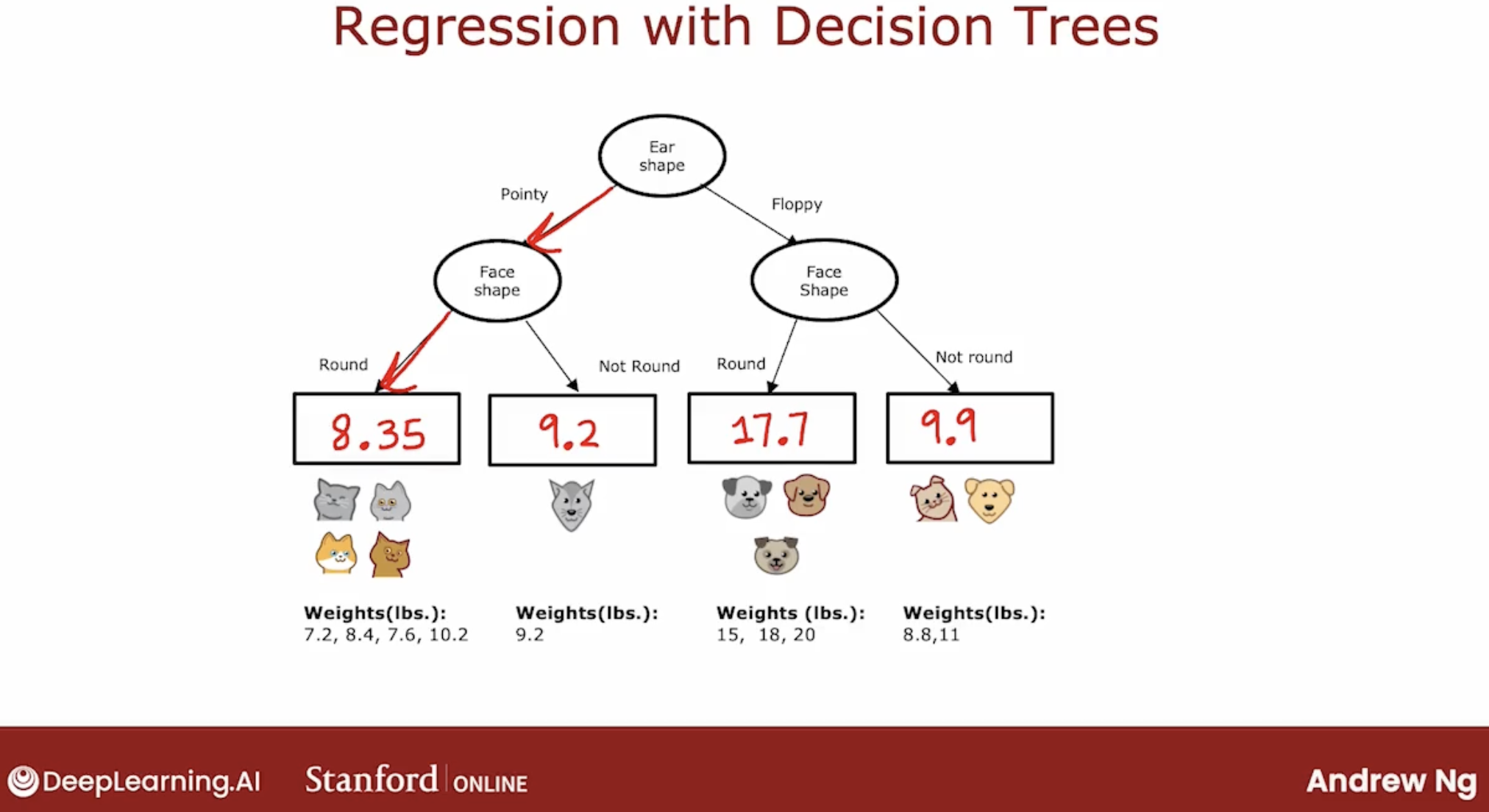
What is regression tree? regression tree is a decision tree which output is a number.
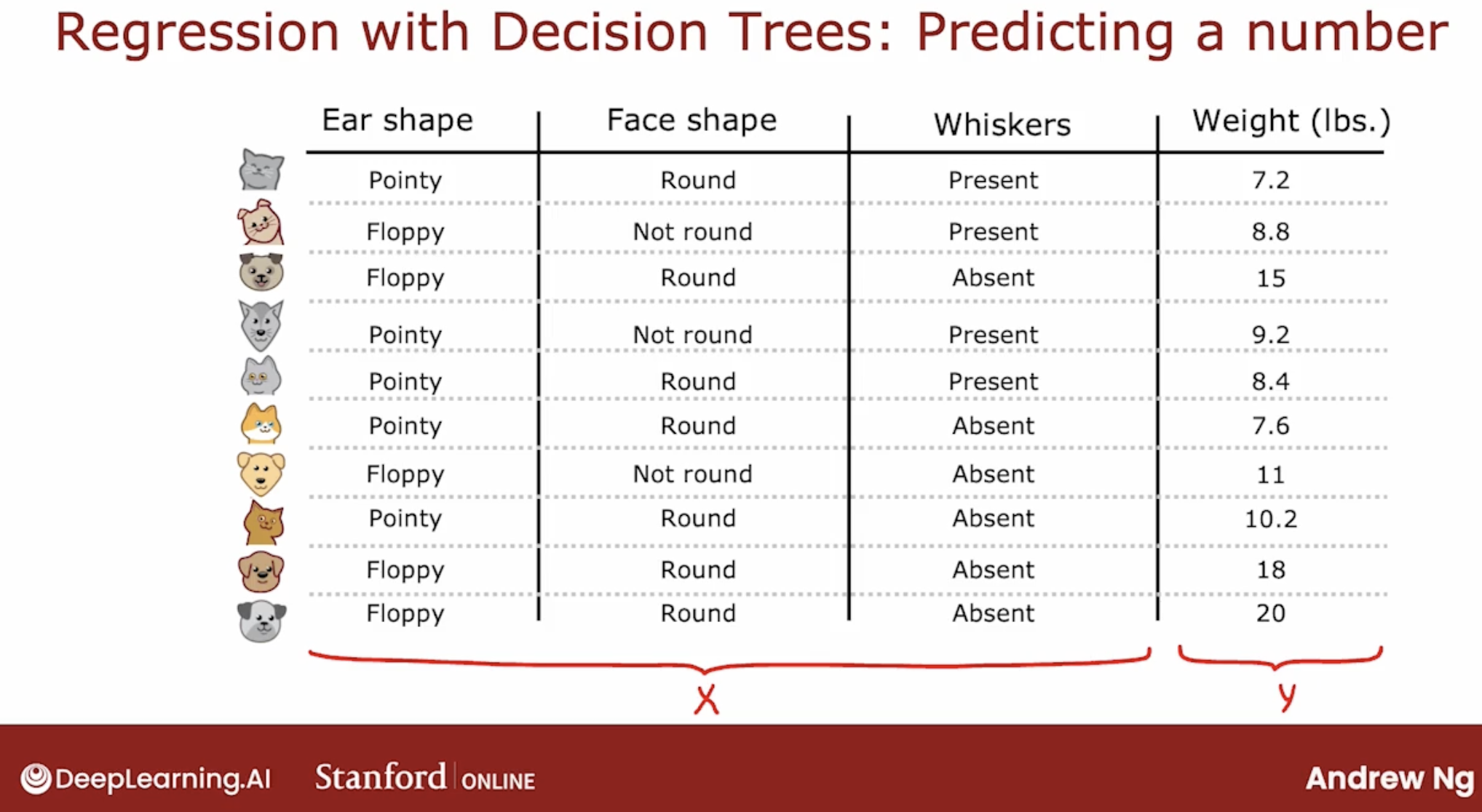
So, how to output a number?
Answer is, use mean of the target value in the leaf node.
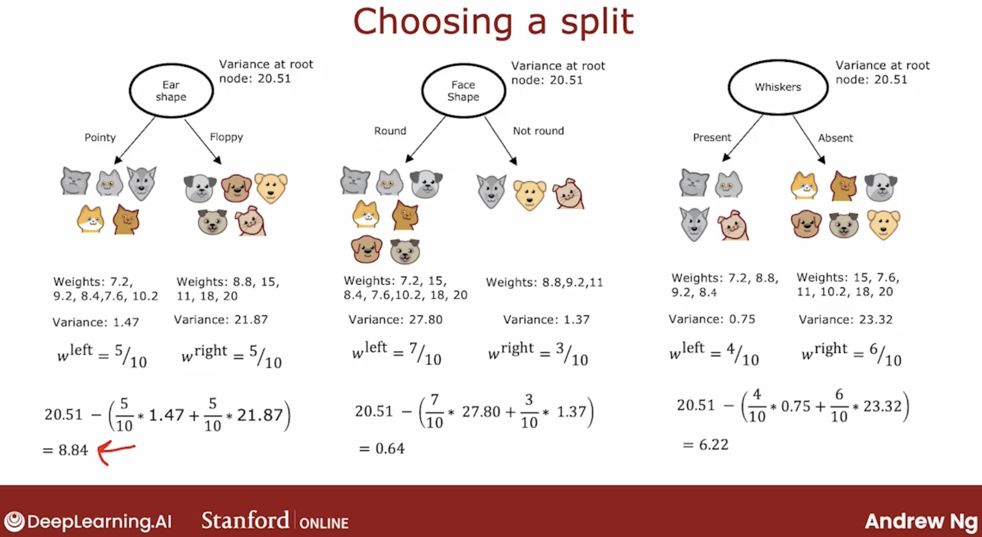
And, there is more importance point is that not choose by largest reduction of entropy, but largest reduction of variance.
more doc:
5 tree ensemble
One of the weaknesses of using a single decision tree is that that decision tree can be highly sensitive to small changes in the data.
One solution to make the algorithm less sensitive or more robust is to build not one decision tree, but to build a lot of decision trees, and we call that a tree ensemble.
weakness: highly sensitive to small changes in the data of single tree.
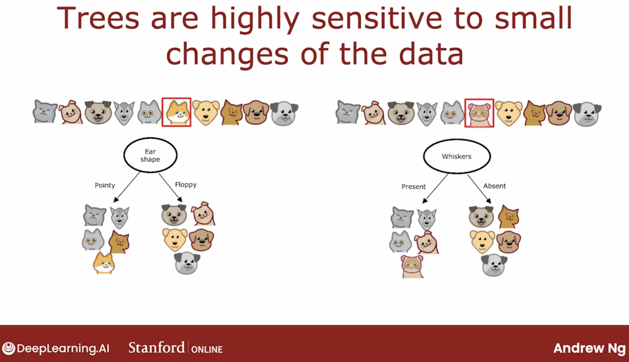
The fact that changing just one training example causes the algorithm to come up with a different split at the root and therefore a totally different tree, that makes this algorithm just not that robust.
so, ensemble tree is mean, if you had this ensemble three trees, each one of these is maybe a plausible way to classify cat versus not cat.
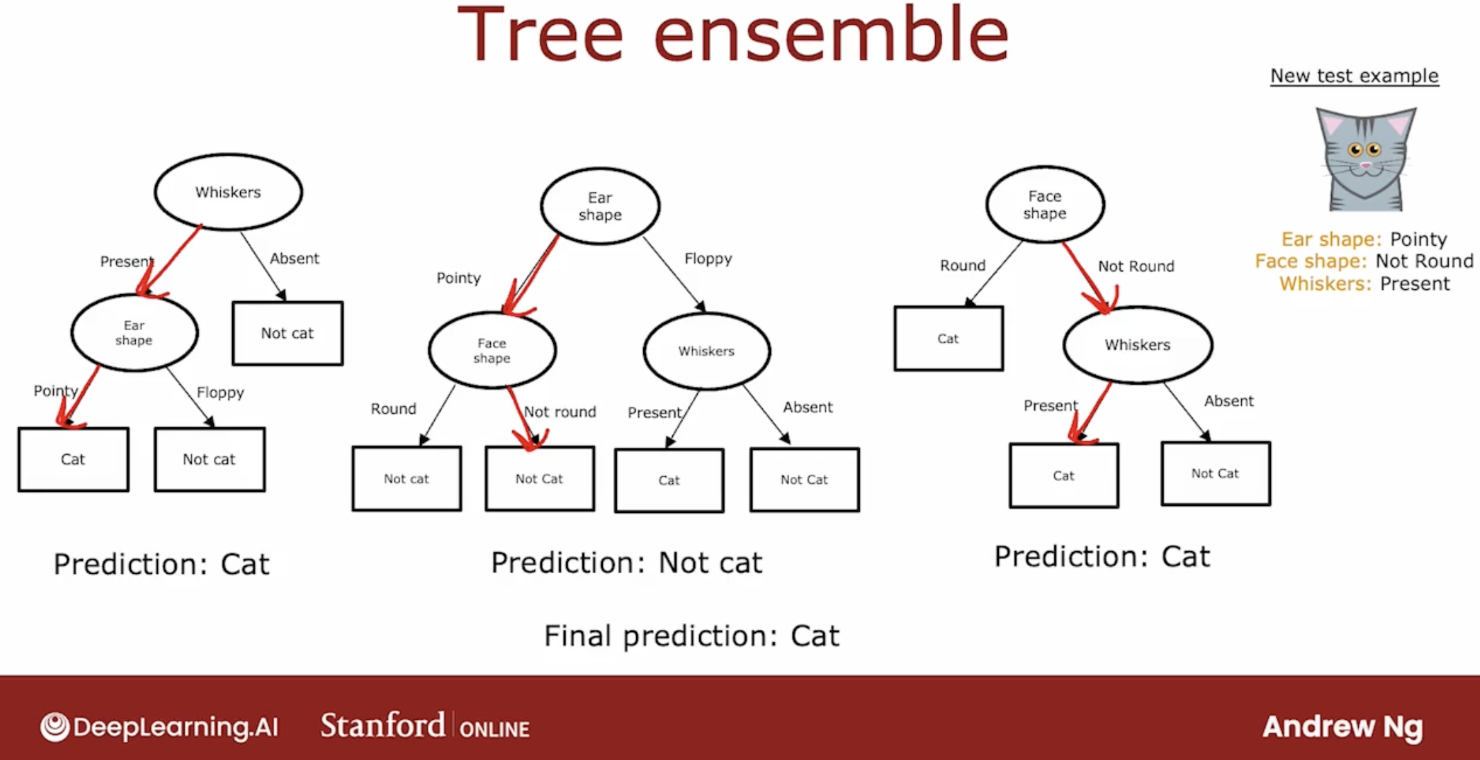
If you had a new test example that you wanted to classify, then what you would do is run all three of these trees on your new example and get them to vote on whether it’s the final prediction.
But how do you come up with all of these different plausible but maybe slightly different decision trees in order to get them to vote?
the answer is a technique from statistics called sampling with replacement.
6 sampling with replacement
Let’s illustrate this with an example.
say you have four tokens, you choosed one token,
and then you need to choose the second token, but the important thing is that you put the first token back into the bag, then you can choose the second token.
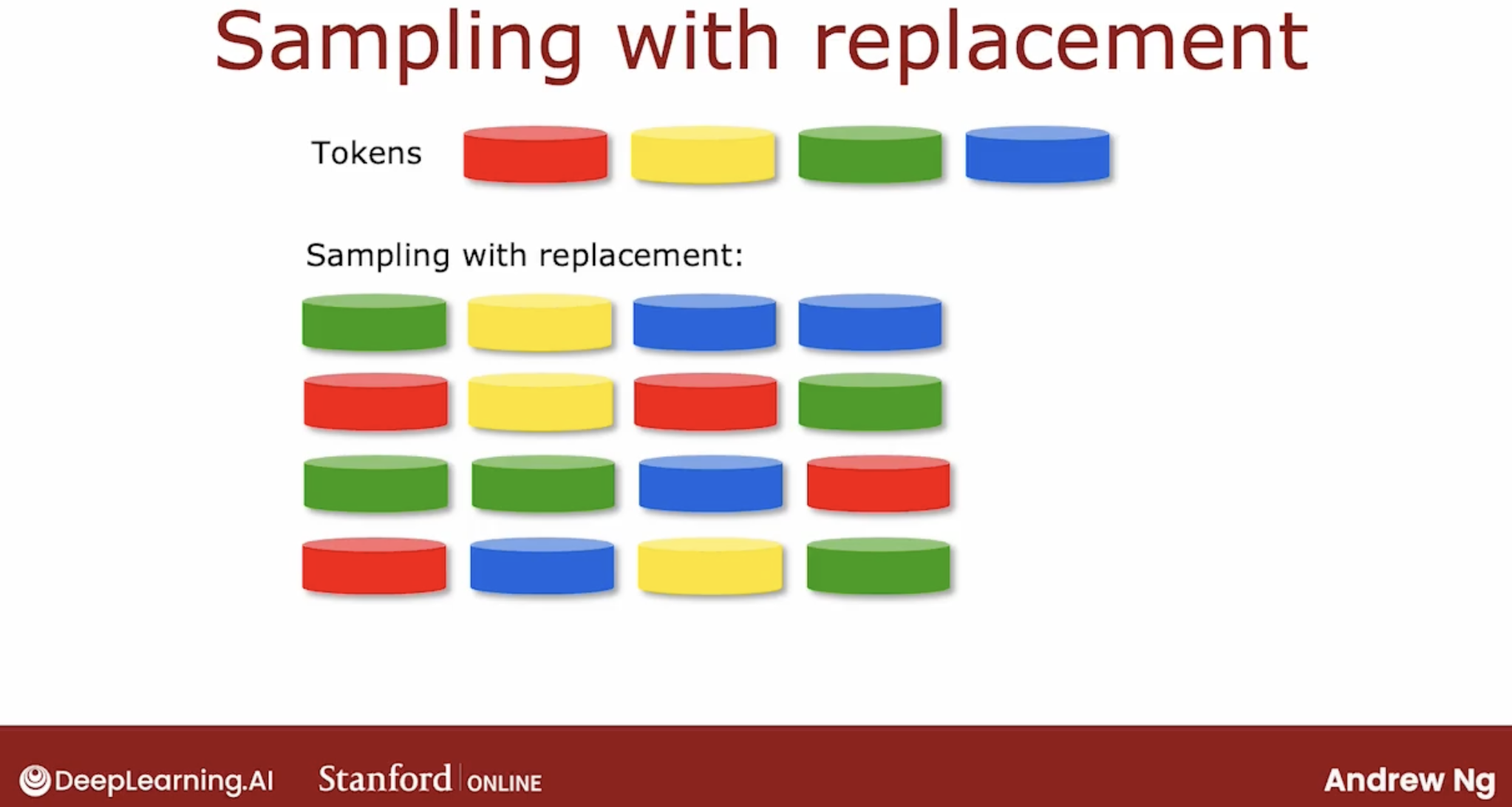
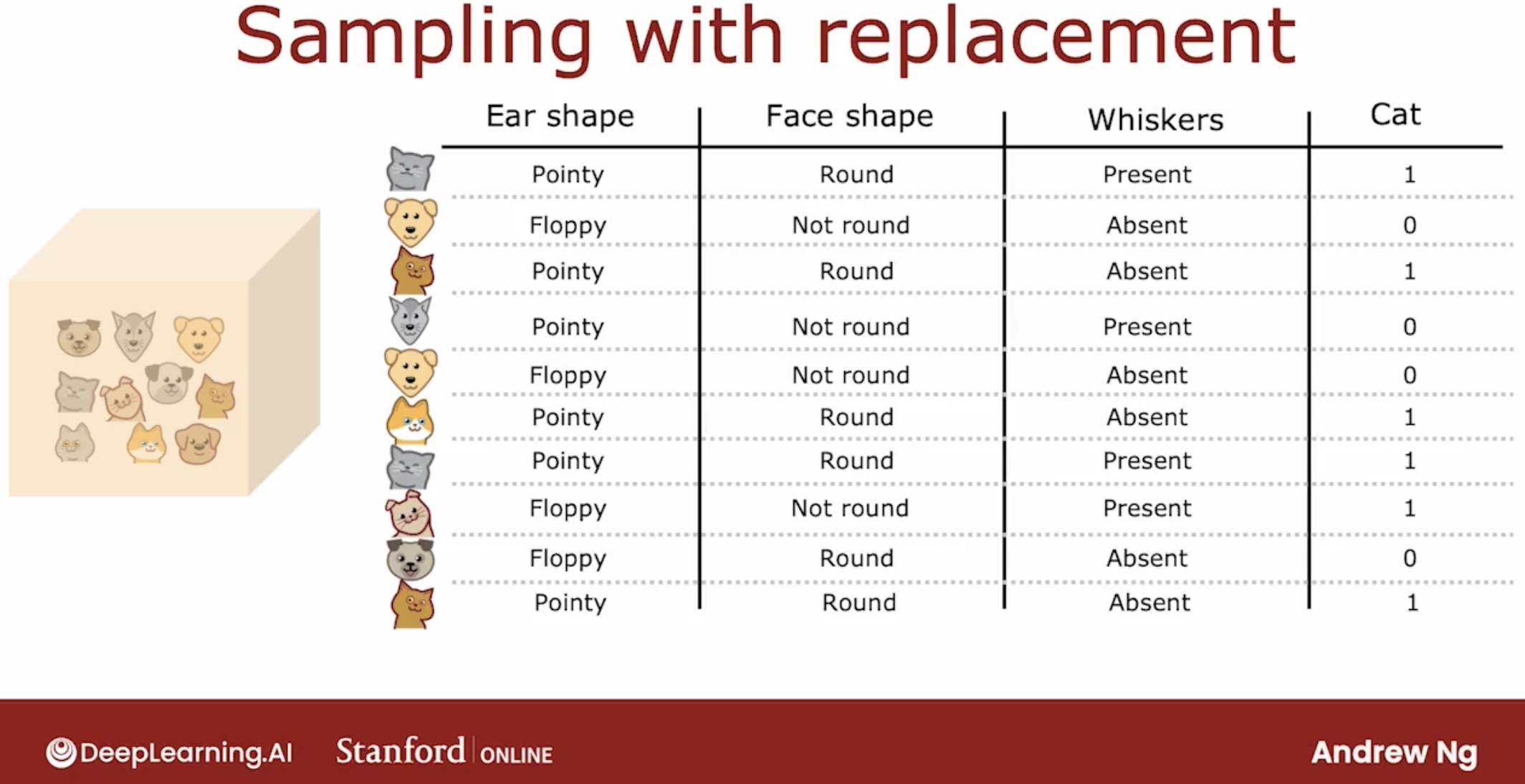
sampling with replacement, the examples number is same as before, but the examples will have high probablity of repeatiion.
The process of sampling with replacement, lets you construct a new training set that’s a little bit similar to, but also pretty different from your original training set.
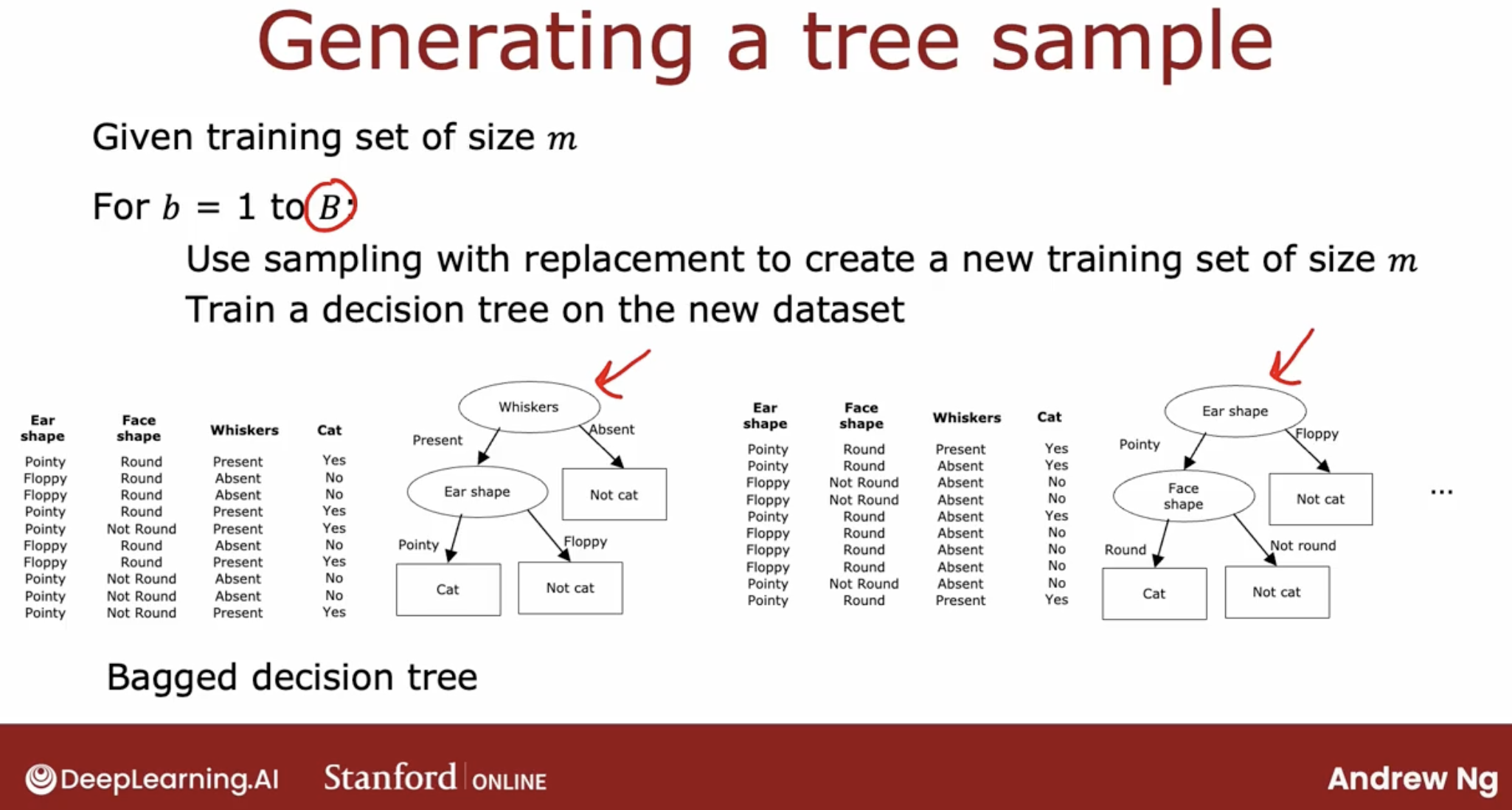
6.1 Bagged decision trees
But there is a caveat, It turns out that setting capital B to be larger, never hurts performance, but beyond a certain point, you end up with diminishing returns and it doesn’t actually get that much better when B is much larger than say 100 or so.
6.2 random forest algorithm
based sampling with replacement, we’re ready to build a tree ensemble algorithm. random forest algorithm.
why need modify this to random forest algorighm?
The key idea is that even with this sampling with replacement procedure sometimes you end up with always using the same split at the root node and very similar splits near the root note.
That didn’t happen in this particular example where a small change the trainings that resulted in a different split at the root note. But for other training sets it’s not uncommon that for many or even all capital B training sets, you end up with the same choice of feature at the root node and at a few of the nodes near the root node.
So there’s one modification to the algorithm to further try to randomize the feature choice at each node that can cause the set of trees and you learn to become more different from each other. So when you vote them, you end up with an even more accurate prediction.
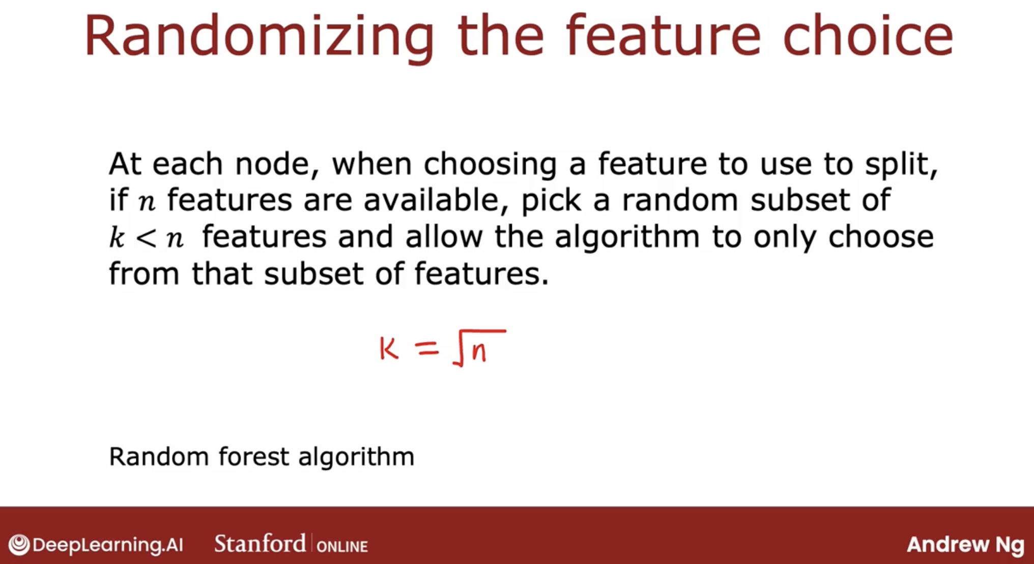
about K value:
When N is large, say n is Dozens or 10’s or even hundreds. A typical choice for the value of K would be to choose it to be square root of N, In our example we have only three features and this technique tends to be used more for larger problems with a larger number of features.
more doc:
7 Boost
7.1 what is boost?
When sampling, instead of picking from all m examples of equal probability with one over m probability, let’s make it more likely that we’ll pick misclassified examples that the previously trained trees do poorly on.
In training and education, there’s an idea called deliberate practice.
For example, if you’re learning to play the piano and you’re trying to master a piece on the piano rather than practicing the entire say five minute piece over and over, which is quite time consuming.
If you instead play the piece and then focus your attention on just the parts of the piece that you aren’t yet playing that well in practice those smaller parts over and over. Then that turns out to be a more efficient way for you to learn to play the piano well.
And so this idea of boosting is similar. We’re going to look at the decision trees, we’ve trained so far and look at what we’re still not yet doing well on. And then when building the next decision tree, we’re going to focus more attention on the examples that we’re not yet doing well.
So rather than looking at all the training examples, we focus more attention on the subset of examples is not yet doing well on and get the new decision tree, the next decision tree reporting ensemble to try to do well on them.
And this is the idea behind boosting and it turns out to help the learning algorithm learn to do better more quickly.
So in detail, we will look at this tree that we have just built and go back to the original training set. Notice that this is the original training set, not one generated through sampling with replacement. And we’ll go through all ten examples and look at what this learned decision tree predicts on all ten examples.
So this fourth most column are their predictions and put a checkmark across next to each example, depending on whether the trees classification was correct or incorrect.
So what we’ll do in the second time through this loop is we will sort of use sampling with replacement to generate another training set of ten examples. But every time we pick an example from these ten will give a higher chance of picking from one of these three examples that were still misclassifying. And so this focuses the second decision trees attention via a process like deliberate practice on the examples that the algorithm is still not yet doing that well.
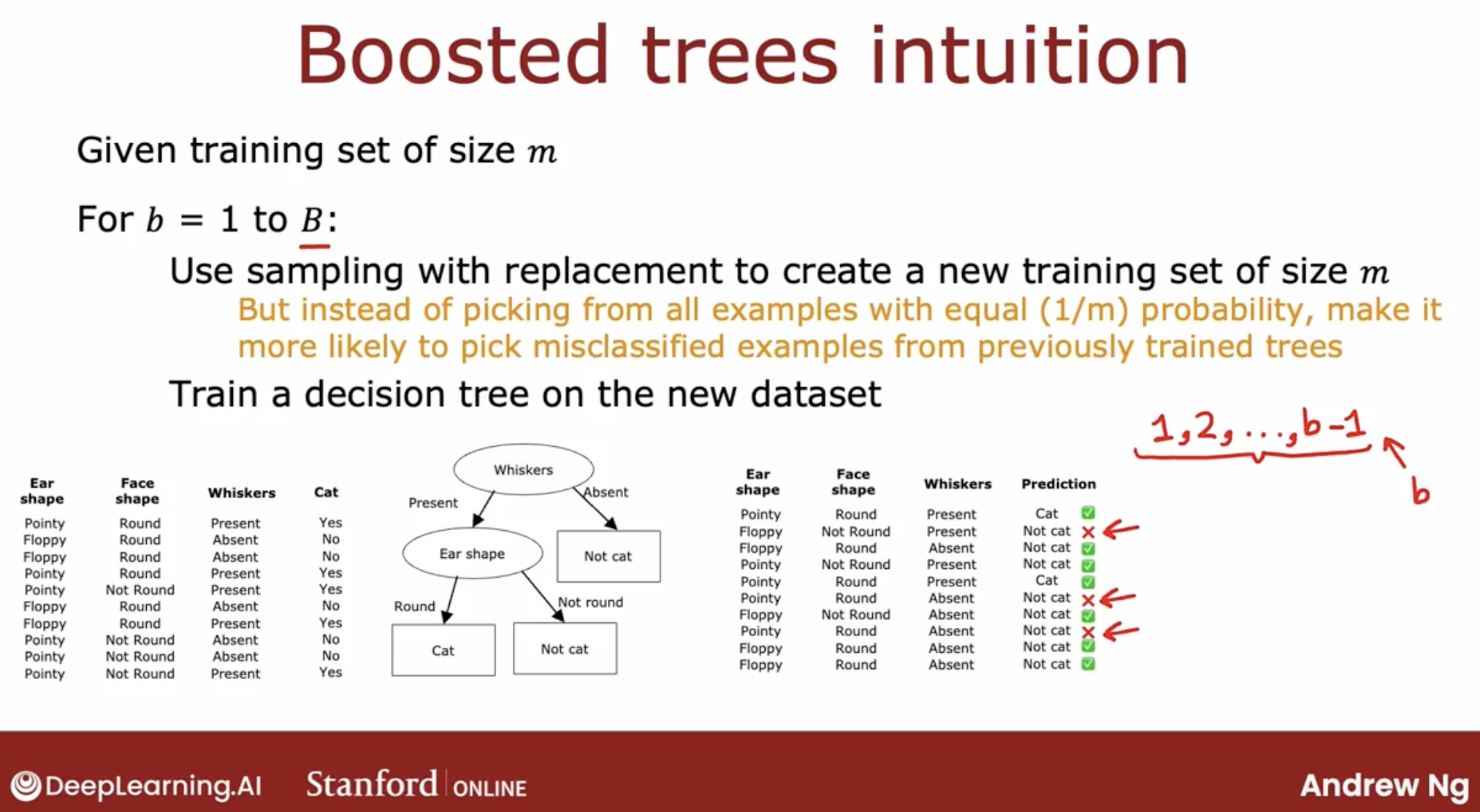
And the boosting procedure will do this for a total of B times where on each iteration, you look at what the ensemble of trees for trees 1, 2 up through (b- 1), are not yet doing that well on.
And when you’re building tree number b, you will then have a higher probability of picking examples that the ensemble of the previously sample trees is still not yet doing well on.
7.2 boosting algorithm
of different ways of implementing boosting the most widely used one today is XGBoost. Gradient Boosting model.
XGBoost has many advantage, and it’s easy to code.
8 difference between decision tree and neural network
different usage scenariese
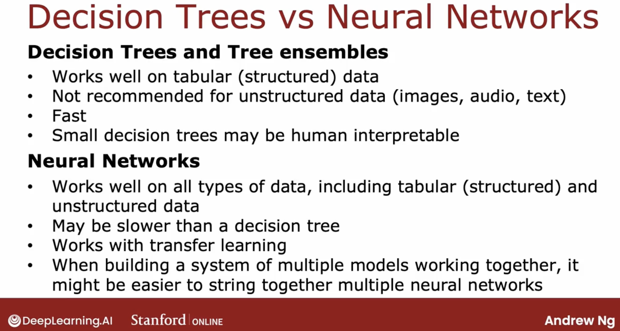
Finally, if you’re building a system of multiple machine learning models working together, it might be easier to string together and train multiple neural networks than multiple decision trees.
The reasons for this are quite technical and you don’t need to worry about it for the purpose of this course. But it relates to that even when you string together multiple neural networks you can train them all together using gradient descent. Whereas for decision trees you can only train one decision tree at a time.