【Meachine Learning】12 Clustering
1 clustering intuition
1.1 classification vs clustering
In supervised learning, the dataset included both the inputs x as well as the target outputs y.
In contrast, in unsupervised learning, you are given a dataset like this with just x, but not the labels or the target labels y.
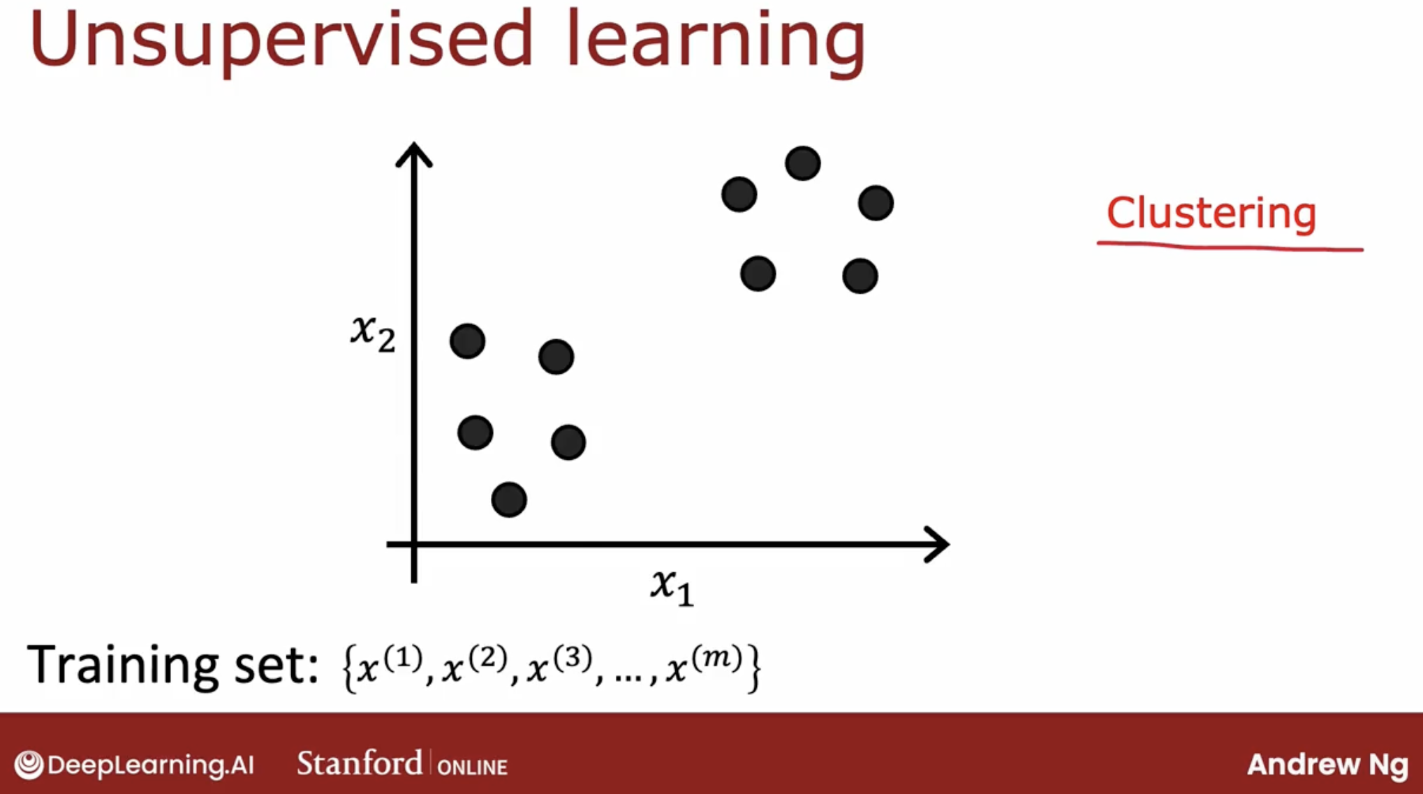
That’s why when I plot a dataset, it looks like this, with just dots rather than two classes denoted by the x’s and the o’s. Because we don’t have target labels y, we’re not able to tell the algorithm what is the “right answer, y” that we wanted to predict.
Instead, we’re going to ask the algorithm to find something interesting about the data, that is to find some interesting structure about this data.
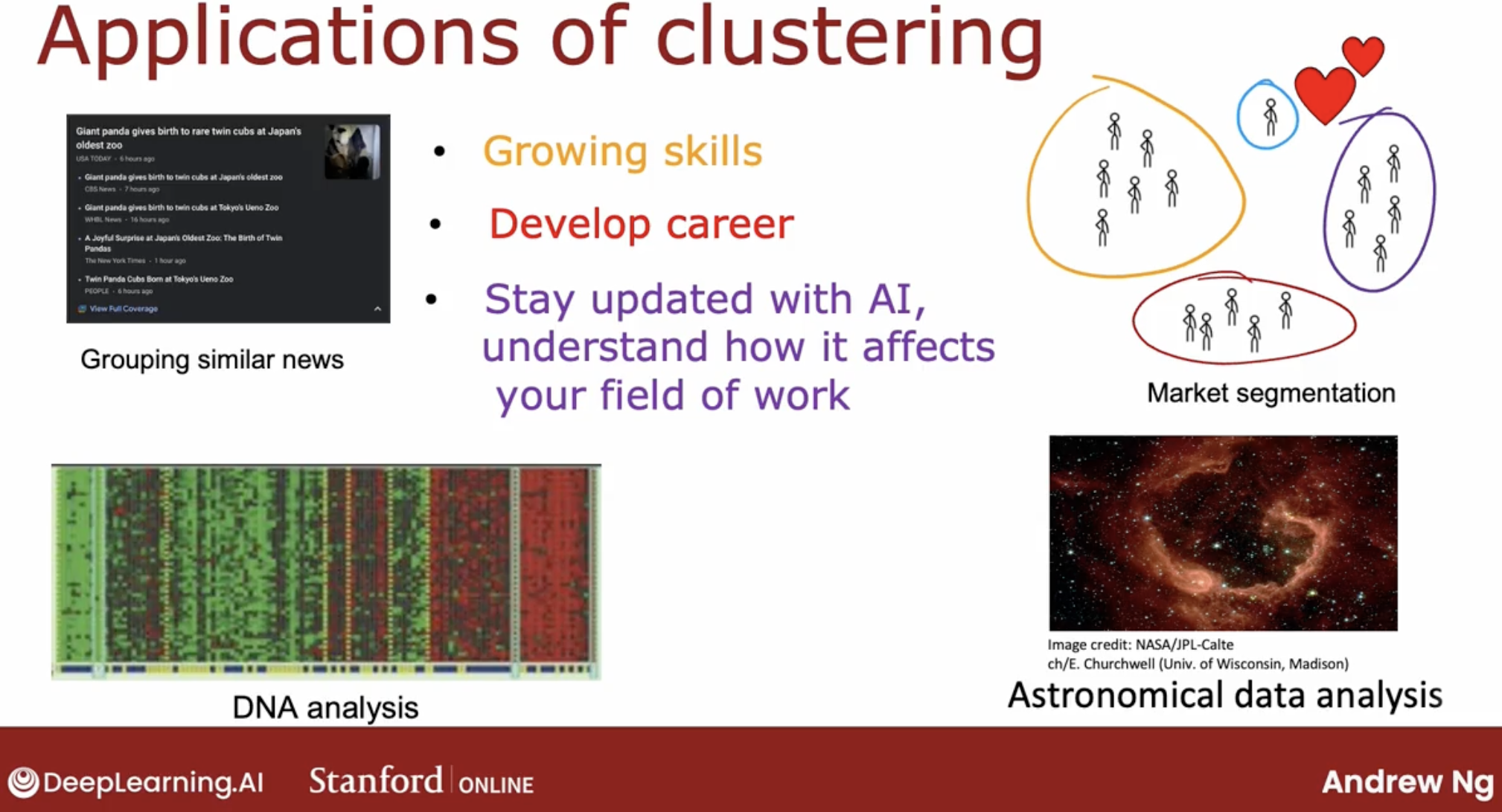
1.2 some more clustering applications
2 K-means clustering
2.1 intuition
What’s K-means clustering?
Let’s say we have a dataset with 1000 points, and we want to find out 2 clusters.
- first, we randomly pick 2 points as the centers of the clusters.
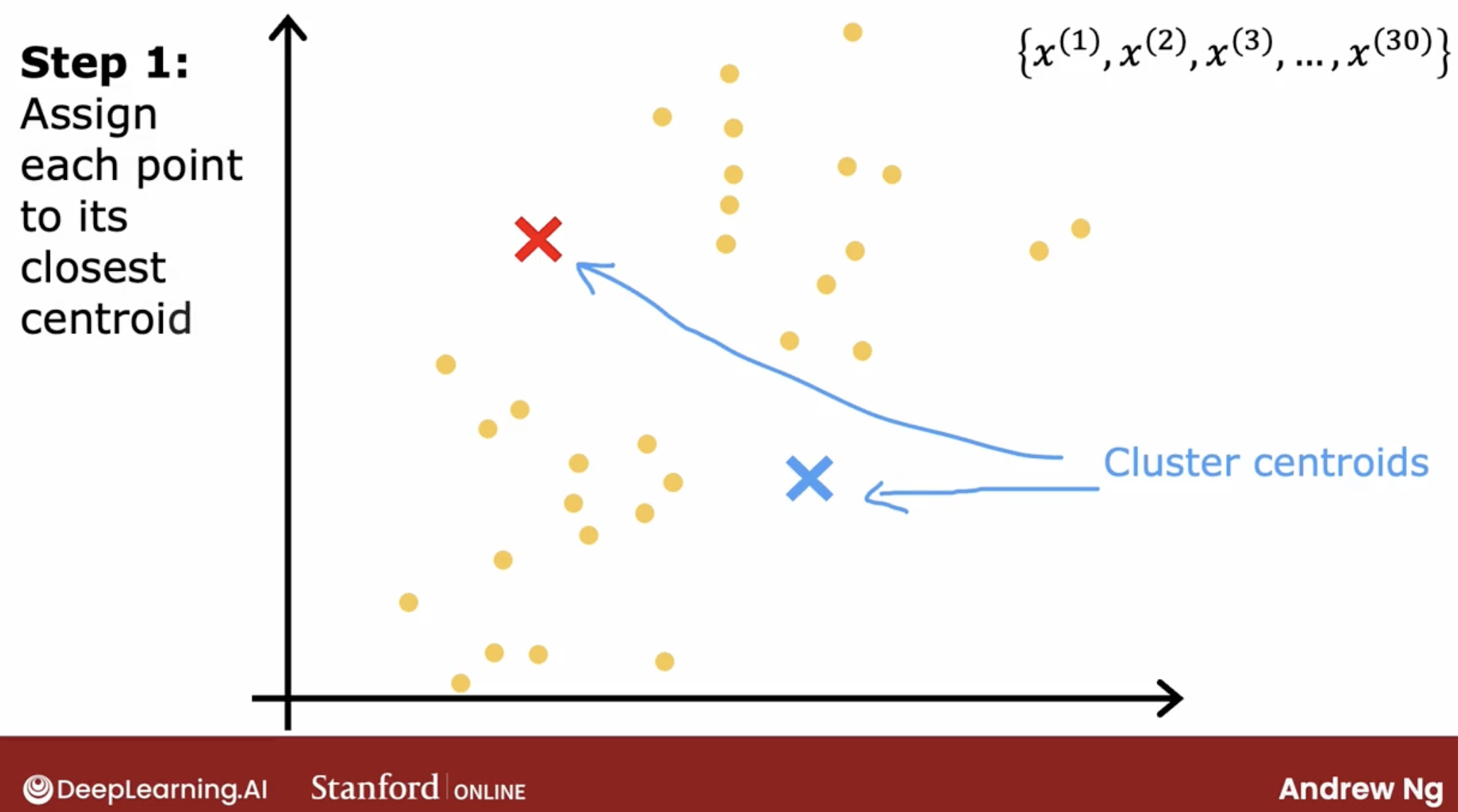
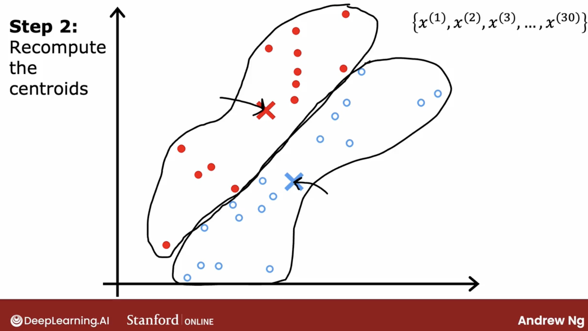
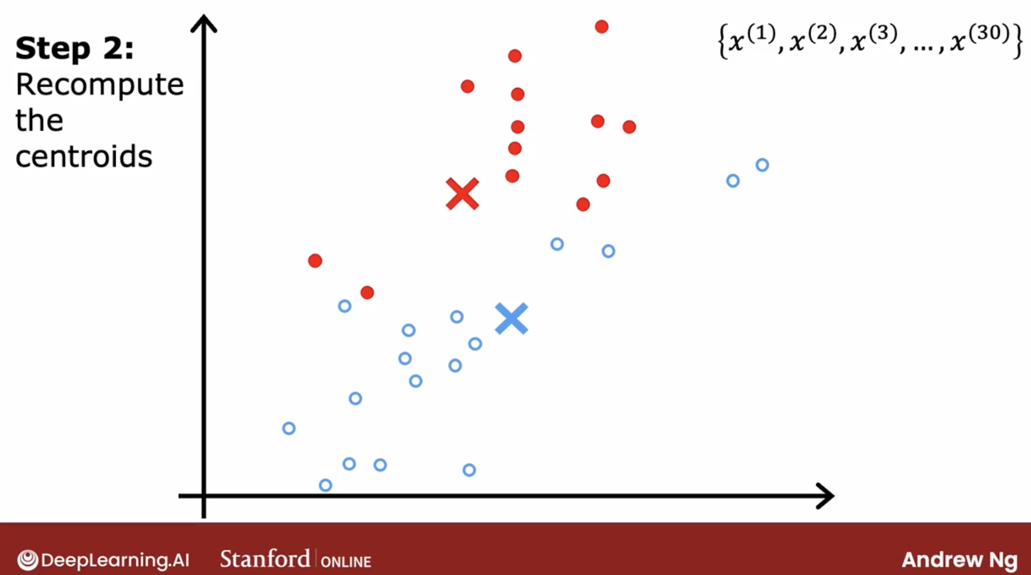
- second, we assign each point to the closest center.
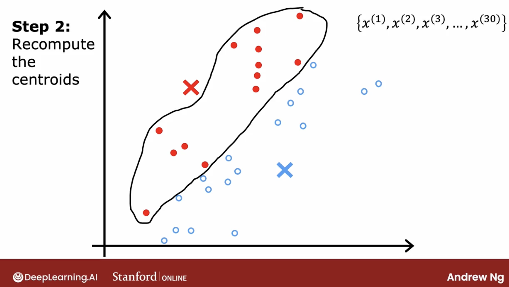
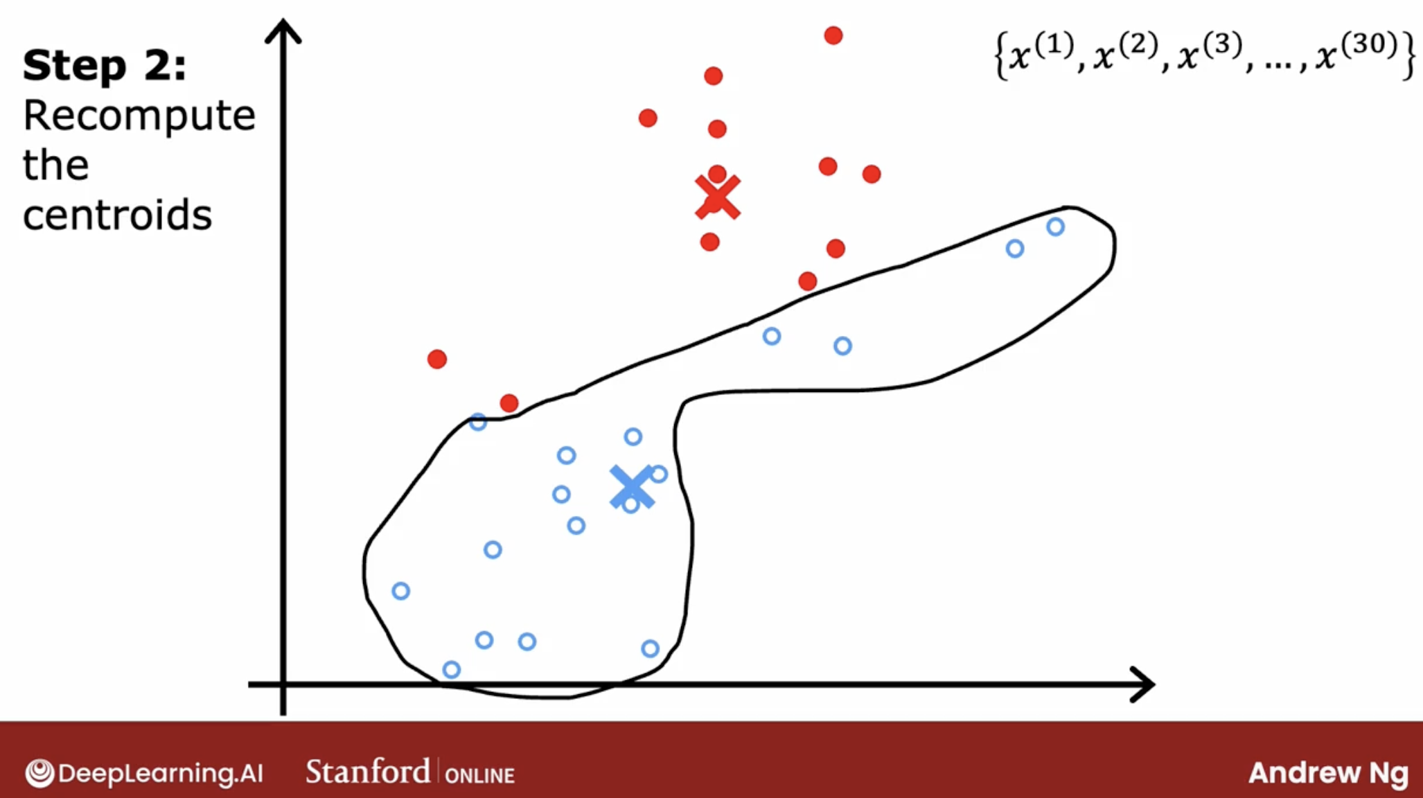
- third, we recalculate the centers of the clusters, and set the two centers as the new centers.
- fourth, we repeat the second and third steps until the centers don’t change anymore.
 …
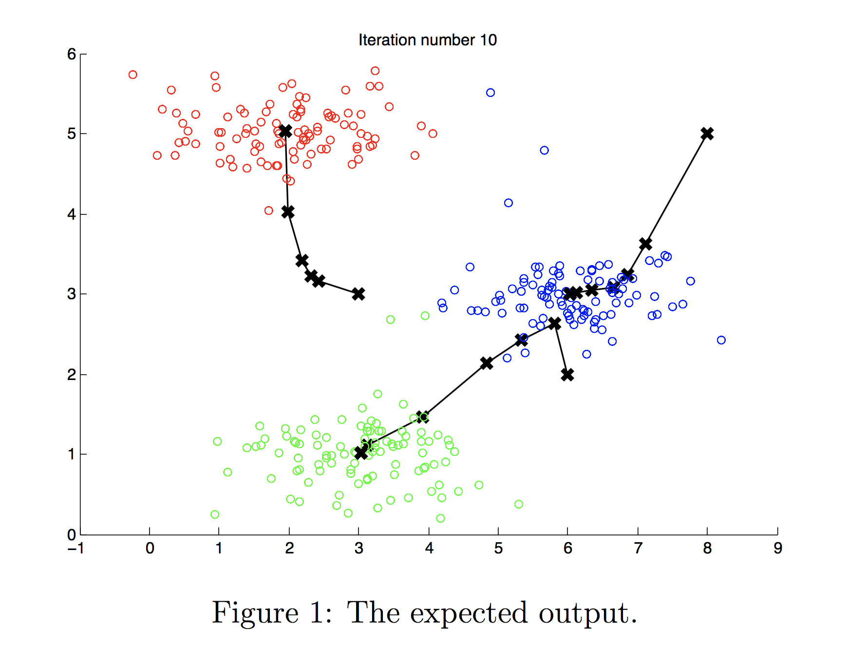
… - at the end, we have 2 clusters. just like the picture below. Note the picture below is 3 clusters., but it’s the same idea.
So, summary, K-means clustering will repeatedly do two different things:
- randomly pick two points as two cluster centroids
- repeat:
- assign points to cluster centroids
- move cluster centroids to the averange of all its points
2.2 algorithm intuition
2.2.1 k-mean algorithm
So, here is the algorithm intuition.
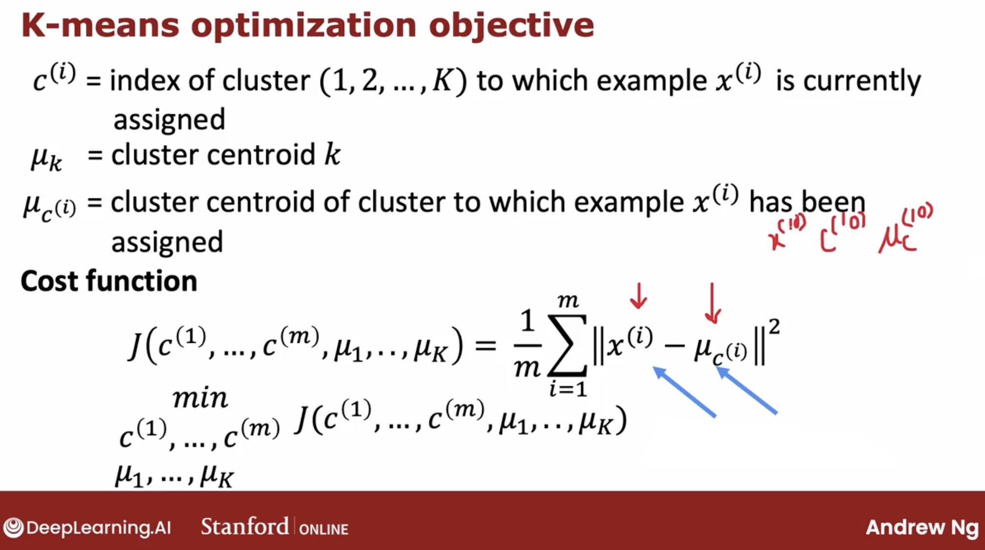
- we have $K$ clusters, and we use $\mu_K$ to represent the centroid of cluster $K$.
- $K$ must less than the $m$ which is the number of points.
- $\mu_K$ is a vector of $x^{(1)}, x^{(2)}, …, x^{(i)}$
- In order to choose the cluster centroids, the most common way is to randomly pick K training examples.
- compute the distance between each point and each centroid.
- $||x^{(i)} - \mu_j||^2$ is the distance of $x^{(i)}$ and $x^{(i)}$, called L2-norm.
2.2.2 local minima
And, there has a common bias in the K-means algorithm, called local minima.
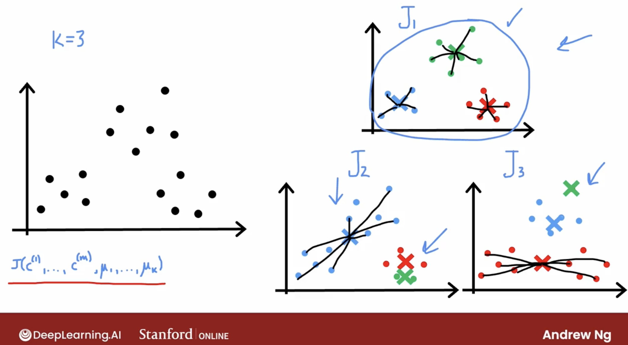
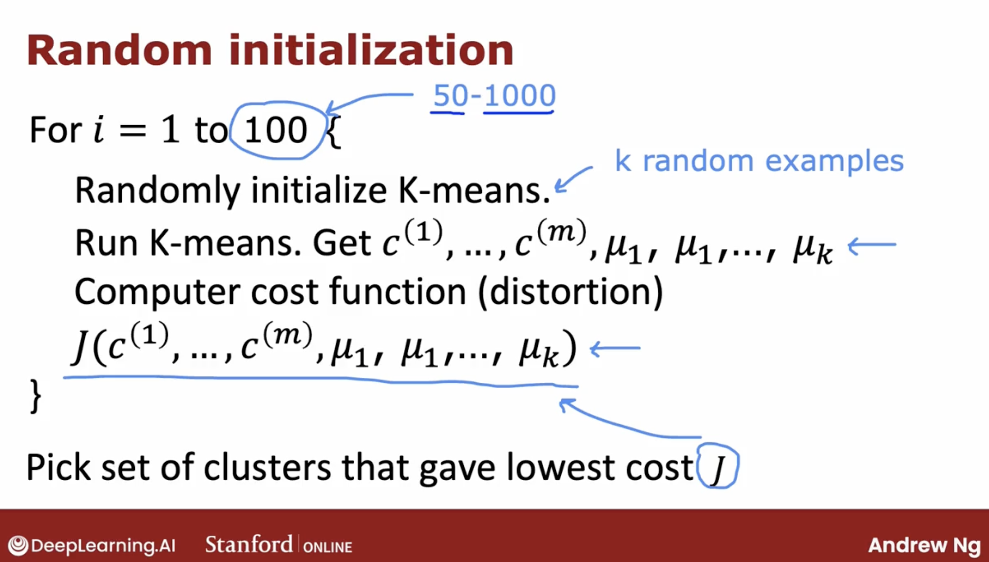
So, one other thing you could do with the K-means algorithm is to run it multiple times and then to try to find the best local optima.
then, what multiple times is?
I plugged in the number up here as 100. When I’m using this method, doing this somewhere between say 50 to 1000 times would be pretty common. Where, if you run this procedure a lot more than 1000 times, it tends to get computational expensive. And you tend to have diminishing returns when you run it a lot of times.
Whereas trying at least maybe 50 or 100 random initializations, will often give you a much better result than if you only had one shot at picking a good random initialization.
2.2.3 k-mean cost function
2.2.4 how to choose $K$
For a lot of clustering problems, the right value of K is truly ambiguous.
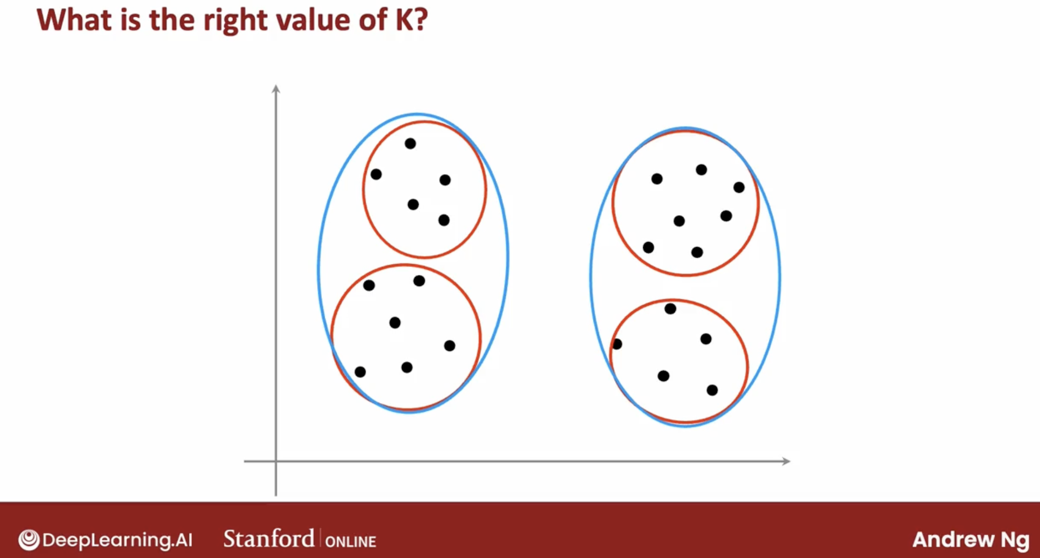
Because clustering is unsupervised learning algorithm you’re not given the quote right answers in the form of specific labels to try to replicate.
There are lots of applications where the data itself does not give a clear indicator for how many clusters there are in it.
some possible method to choose $K$:
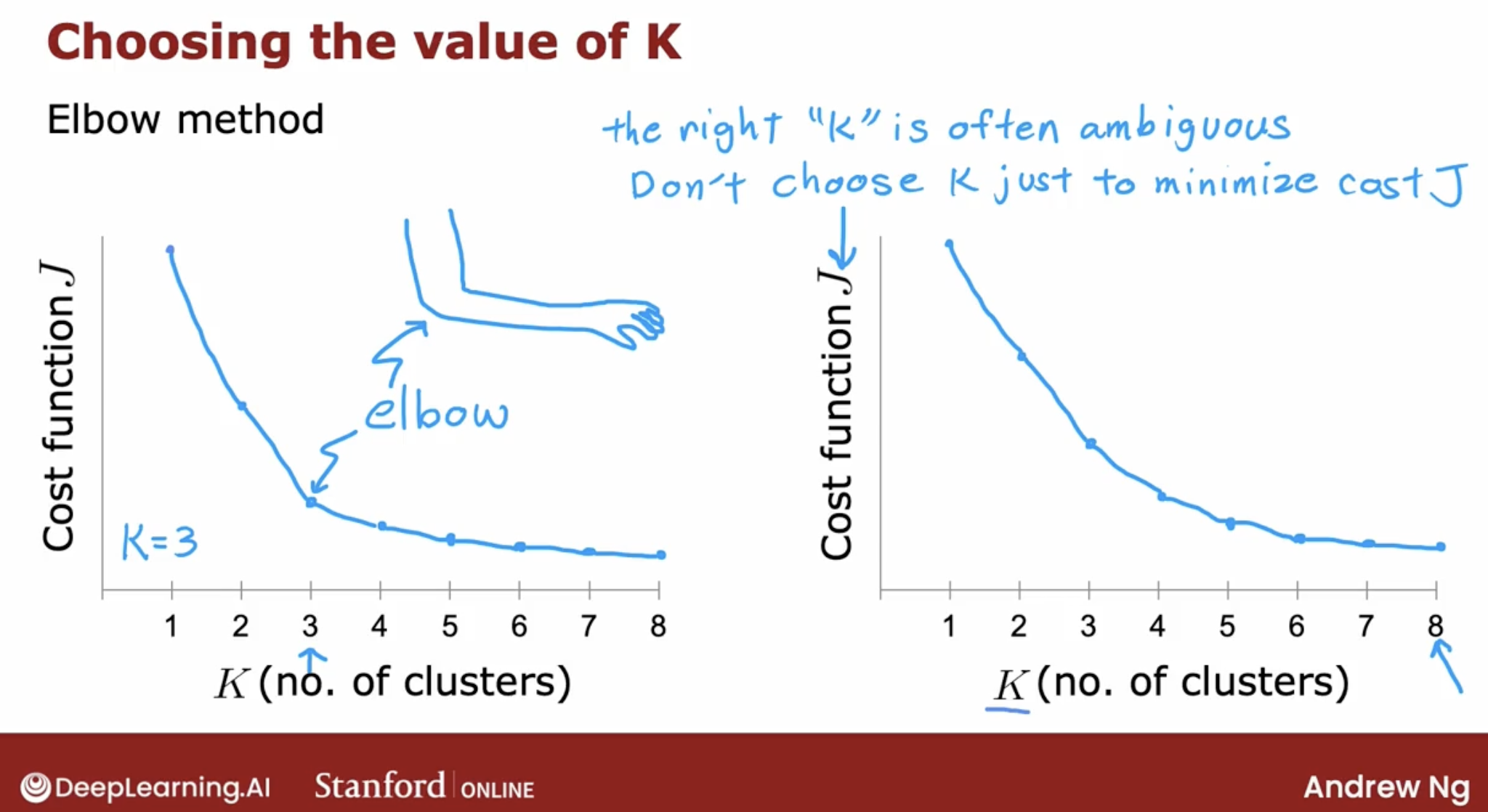
elbow method: a lot of cost functions look like this with just decreases smoothly and it doesn’t have a clear elbow by wish you could use to pick the value of K.
minimum cost function:
- By the way, one technique that does not work is to choose K so as to minimize the cost function J because doing so would cause you to almost always just choose the largest possible value of K because having more clusters will pretty much always reduce the cost function J.
- Choosing K to minimize the cost function J is not a good technique.
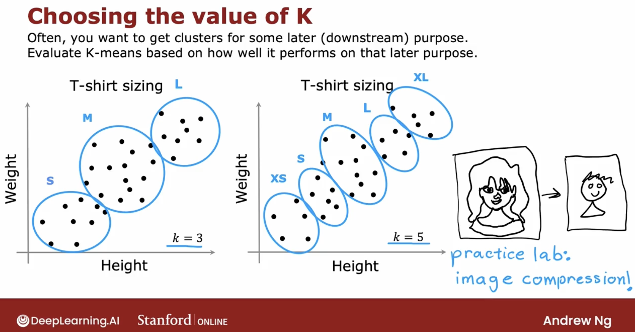
Often you’re running K-means in order to get clusters to use for some later or some downstream purpose. That is, you’re going to take the clusters and do something with those clusters.
What I usually do and what I recommend you do is to evaluate K-means based on how well it performs for that later downstream purpose.
2.3 advantages
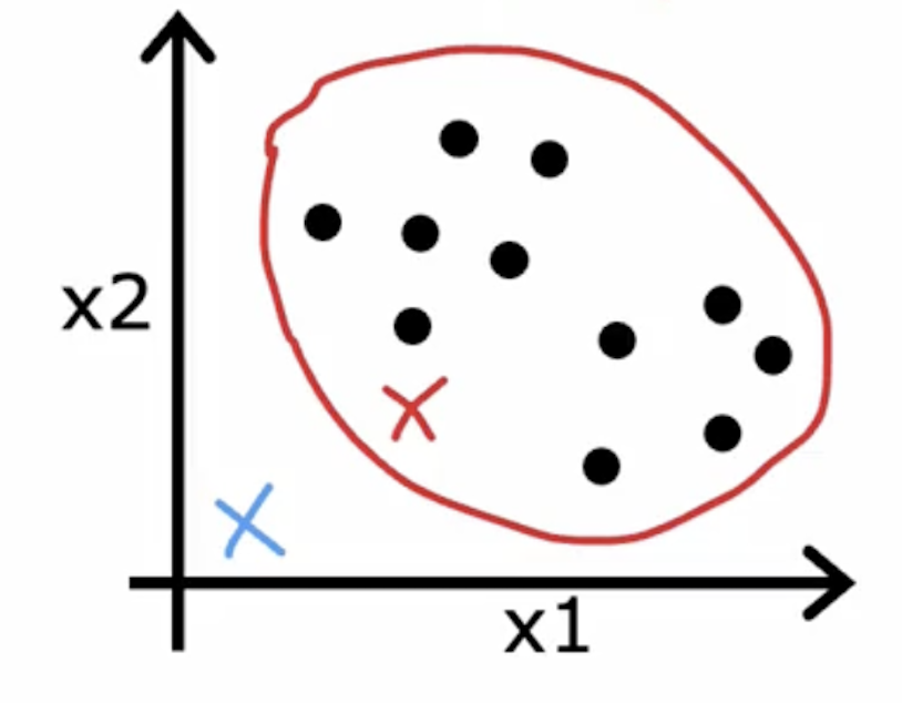
2.3.1 work fine on not well-separated data

This is an example of K-means working just fine and giving a useful results even if the data does not lie in well-separated groups or clusters.
2.4 exceptions
2.4.1 cluster has zero training examples
Now, there is one corner case of this algorithm, which is what happens if a cluster has zero training examples assigned to it.
If that ever happens, the most common thing to do is to just eliminate that cluster. You end up with K minus 1 clusters.
Or if you really, really need K clusters an alternative would be to just randomly reinitialize that cluster centroid and hope that it gets assigned at least some points next time round.
But it’s actually more common when running K-means to just eliminate a cluster if no points are assigned to it.
2.5 code demo
3 Anomaly detection
3.1 intuition
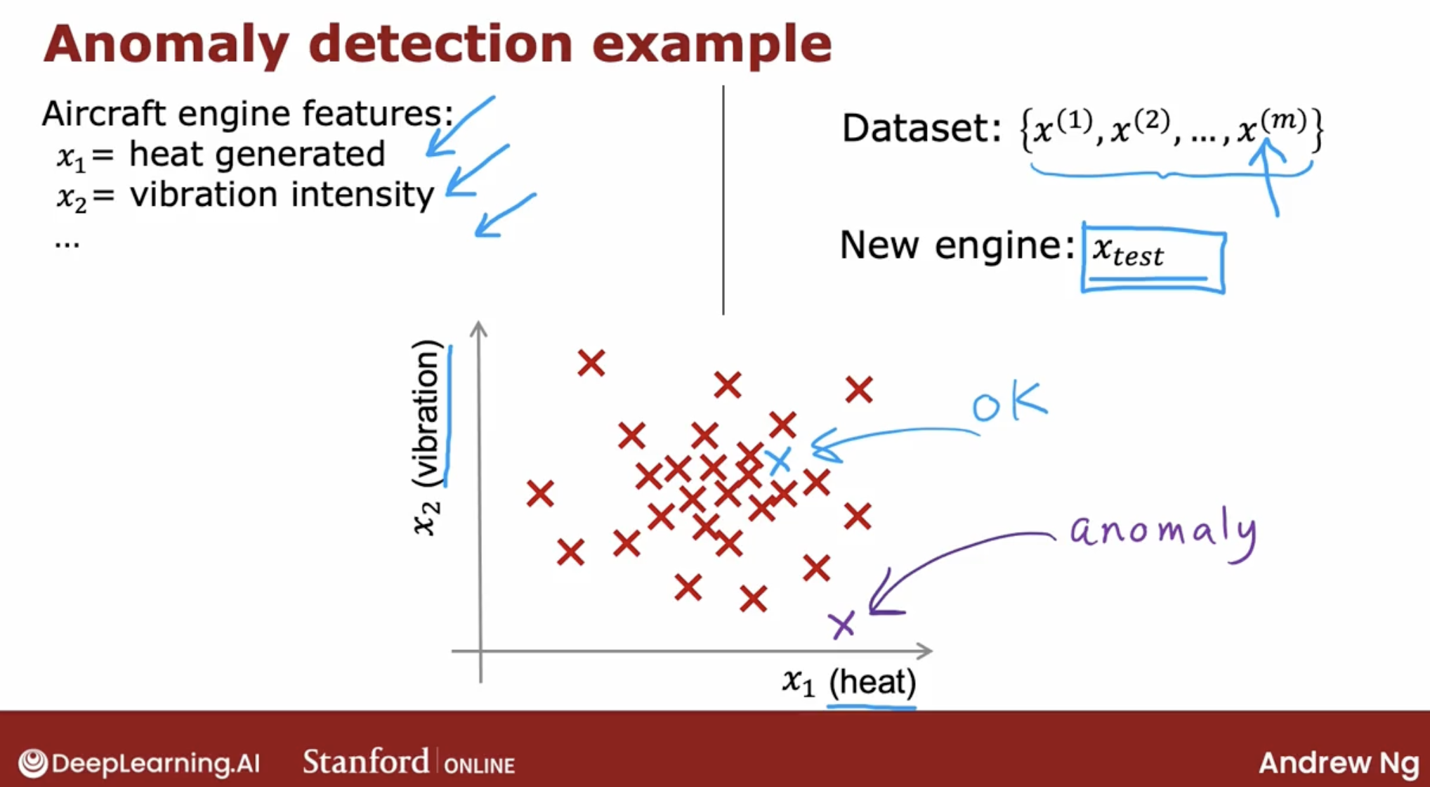
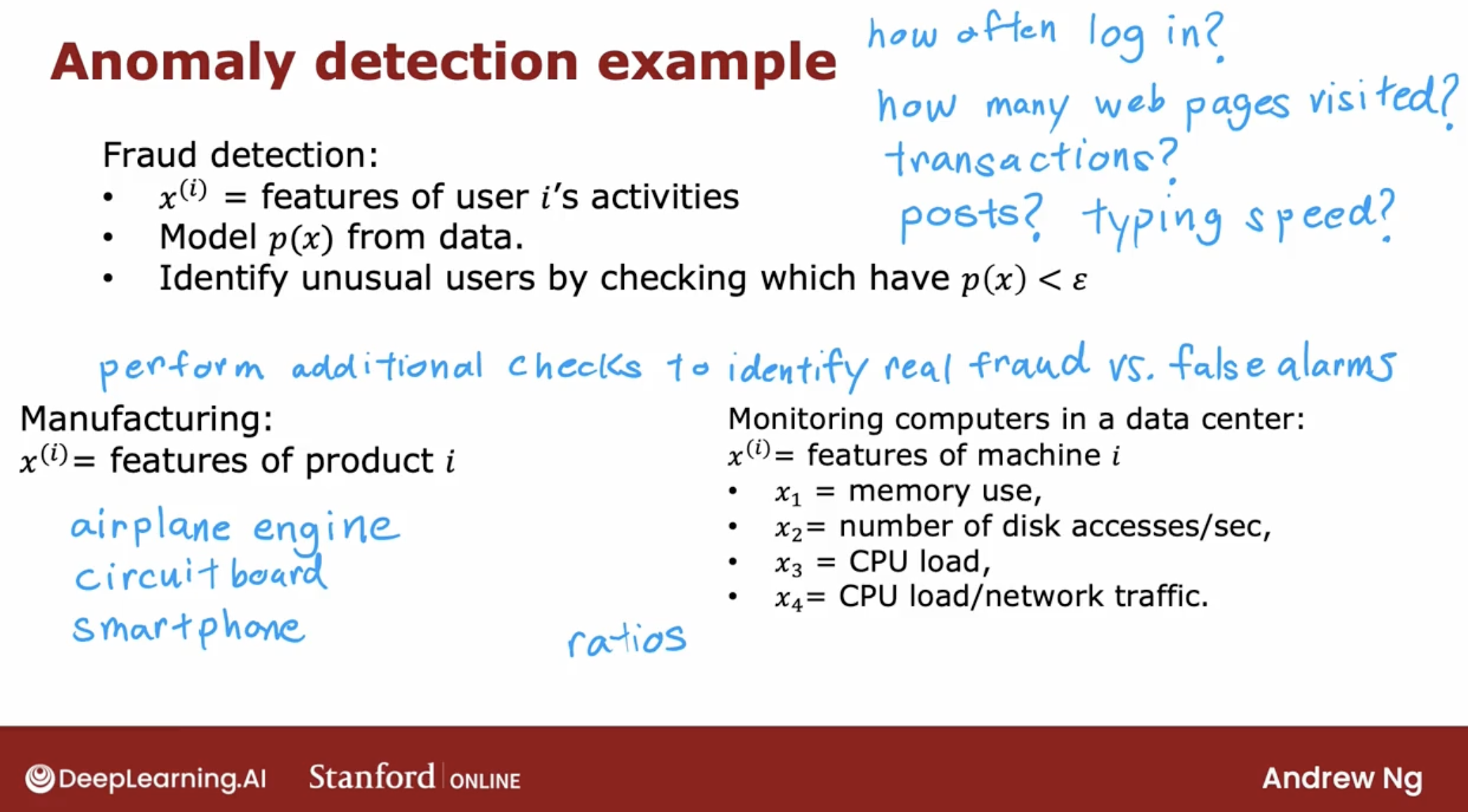
Anomaly detection algorithms look at an unlabeled dataset of normal events and thereby learns to detect or to raise a red flag for if there is an unusual or an anomalous event.
intuition about anomaly detection by aircraft engine.
Anything from an airplane engine to a printed circuit board to a smartphone to a motor, to many, many things to see if you’ve just manufactured the unit that somehow behaves strangely.
Because that may indicate that there’s something wrong with your airplane engine or printed circuit boards or what have you that might cause you to want to take a more careful look before you ship that object to the customer.
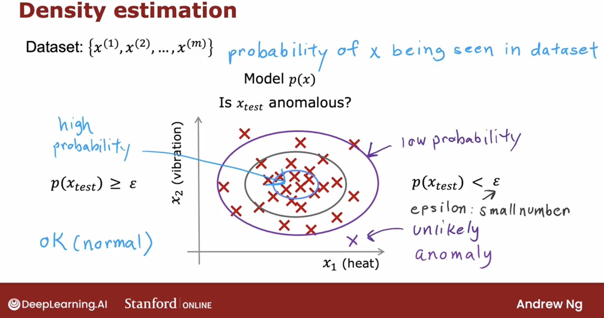
3.2 density estimation
The most common way to carry out anomaly detection is through a technique called density estimation. And what that means is, when you’re given your training sets of these m examples, the first thing you do is build a model for the probability of feature $x_j$.
So, What is the model for the probability of feature $x_j$? Answer is Gaussian distribution.
3.2.1 the probability of feature $x_j$: Gaussian distribution
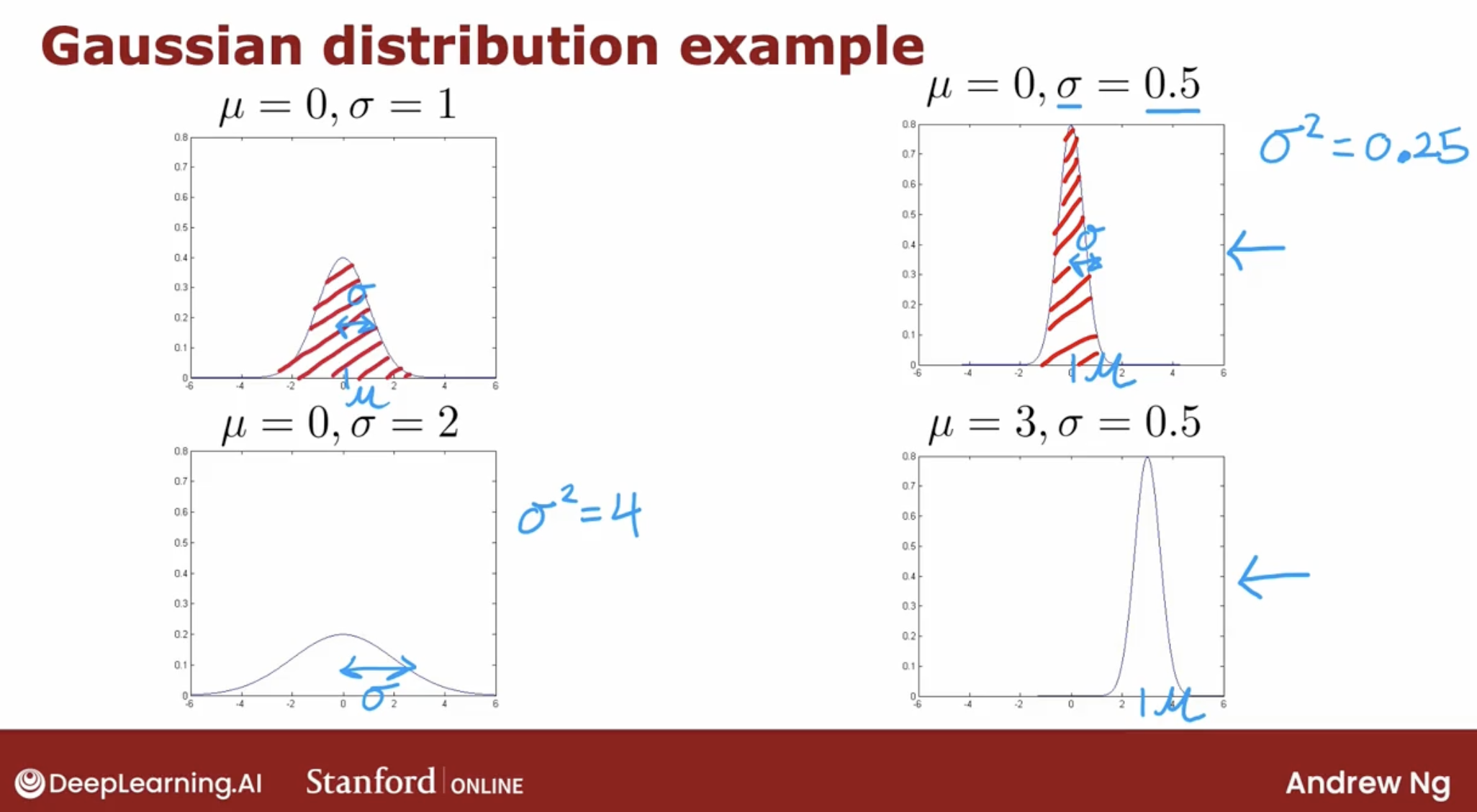
Gaussian distribution or normal distribution or bell-shaped distribution, they mean exactly the same thing.
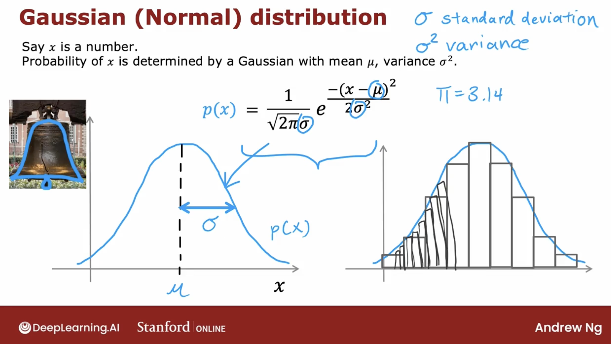
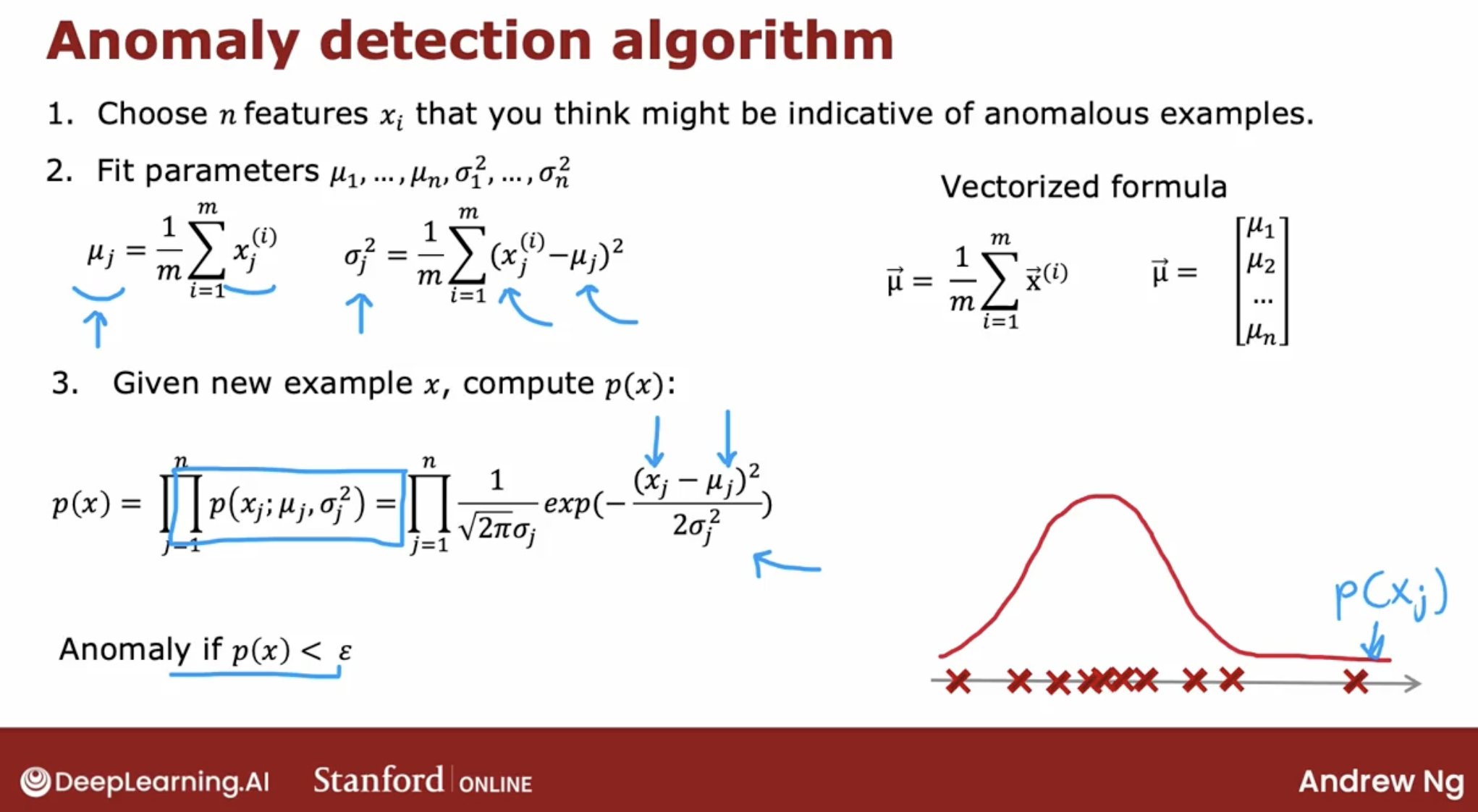
Here is the Gaussian distribution algorithm.
- \[p(x ; \mu,\sigma ^2) = \frac{1}{\sqrt{2 \pi \sigma ^2}}\exp^{ - \frac{(x - \mu)^2}{2 \sigma ^2} }\]
- \[\mu_i = \frac{1}{m} \sum_{j=1}^m x_i^{(j)}\]
- \[\sigma_i^2 = \frac{1}{m} \sum_{j=1}^m (x_i^{(j)} - \mu_i)^2\]
Note: probabilities always have to sum up to one.
3.2.2 the probability of example $x^i$
So, we have a model for the probability of x.
then we say the probability of one example with features$x^1, x^2, … x^n$ is $p(x^1, x^2, …, x^n)$.
and the probability of this example is
\[\prod_{j=1}^n p(x_j ; \mu_j,\sigma_j^2) = p(x_1 ; \mu_1,\sigma_1^2) * p(x_2 ; \mu_2,\sigma_2^2) * ... * p(x_n ; \mu_n,\sigma_n^2)\]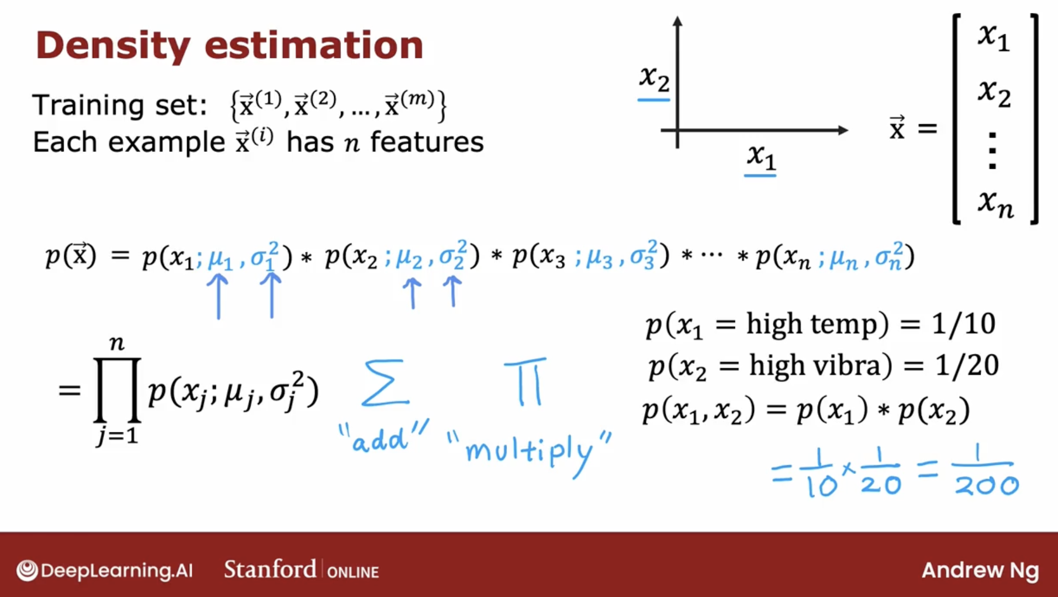
And, let’s see a simple example.
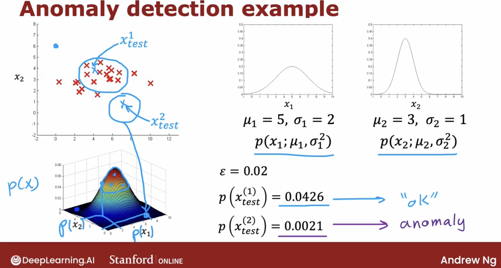
As the image we can see that the final step is to see a p(x) is less than epsilon. And if it is then you flag that it is an anomaly.
3.3 algorithm intuition
3.4 practical optimization
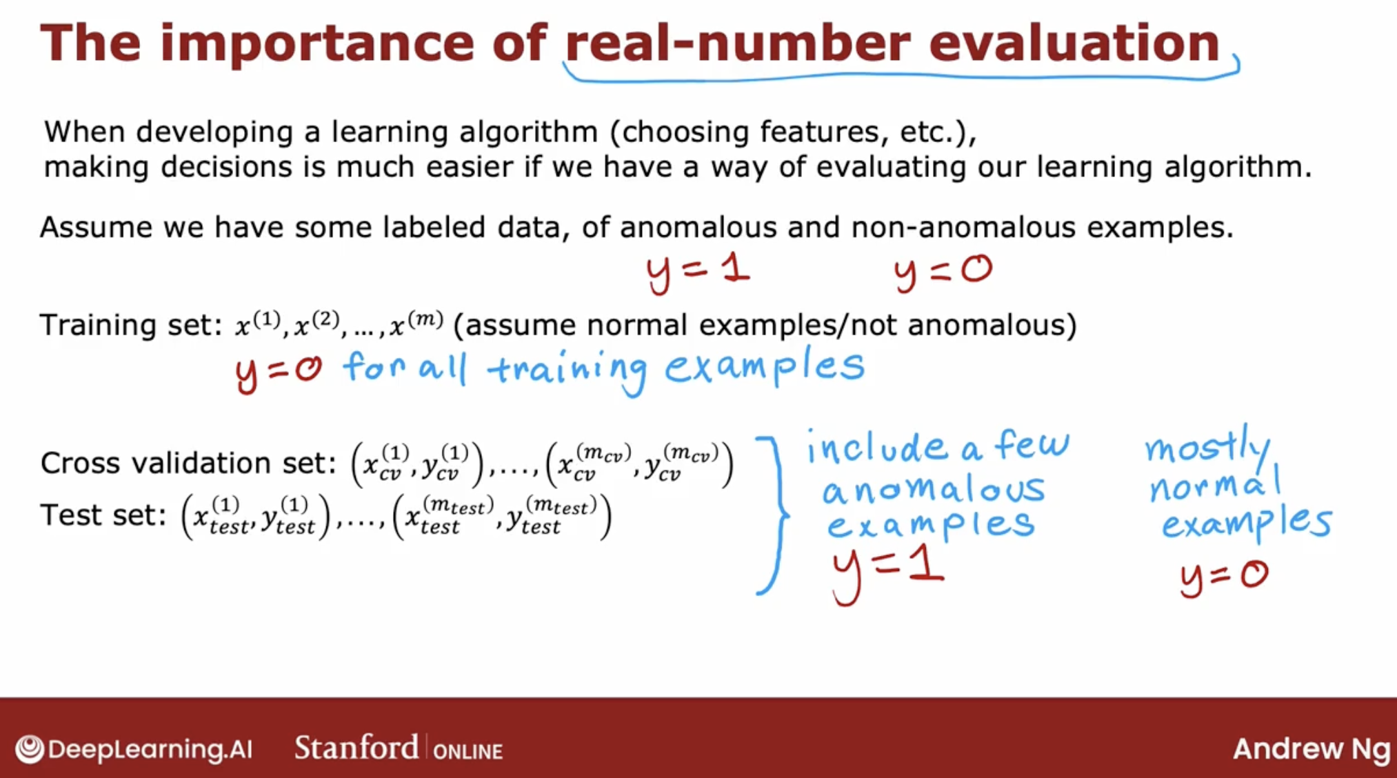
One of the key ideas will be that if you can have a way to evaluate a system, even as it’s being developed, you’ll be able to make decisions and change the system and improve it much more quickly.
etc.
- choosing different features
- trying different values of the parameters like epsilon,
- making decisions about whether or not to change a feature in a certain way
- increase or decrease epsilon or other parameters
- …
And, there are one special function: real-number evaluation.
3.4.1 real-number evaluation
advantages
Notice that this is still primarily an unsupervised learning algorithm because the training sets really has no labels or they all have labels that we’re assuming to be y equals 0 and so we learned from the training set by fitting the Gaussian distributions as you saw in the previous video.
But it turns out if you’re building a practical anomaly detection system, having a small number of anomalies to use to evaluate the algorithm that your cross validation and test sets is very helpful for tuning the algorithm.
disadvantages
But surely you can do, is not give the flawed examples in the cross validation set, or the flawed examples is too small, say 2.
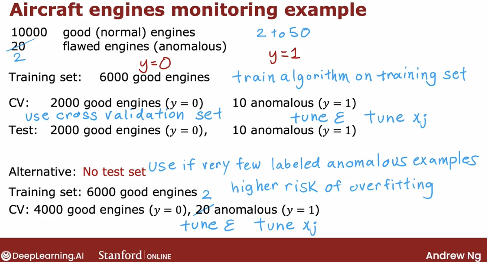
If you have very few flawed engines, so if you had only two flawed engines, then this really makes sense to put all of that in the cross validation set.
The downside of this alternative here is that after you’ve tuned your algorithm, you don’t have a fair way to tell how well this will actually do on future examples because you don’t have the test set.
If this is the case, just be aware that there’s a higher risk that you will have over-fit some of your decisions around Epsilon and choice of features and so on to the cross-validation set and so its performance on real data in the future may not be as good as you were expecting.
summary
The intuition I hope you get is to use the cross-validation set to just look at how many anomalies is finding and also how many normal engines is incorrectly flagging as an anomaly. Then to just use that to try to choose a good choice for the parameter Epsilon.
3.4.2 skew data
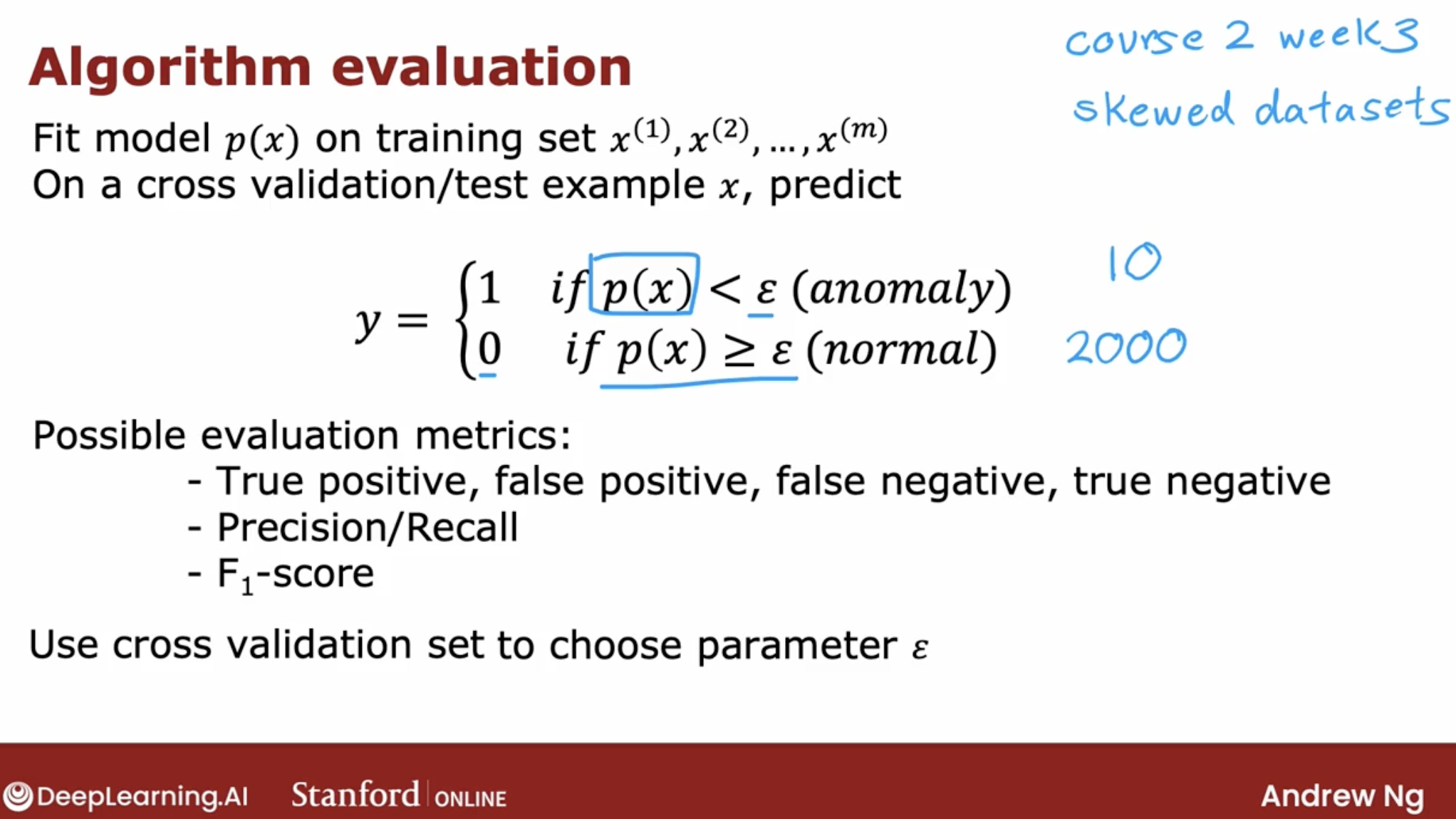
As we can see, the data is skewed. how to deal with it? look at the blog before:
3.4.3 about non-gaussian features
One step that can help your anomaly detection algorithm, is to try to make sure the features you give it are more or less Gaussian.
And if your features are not Gaussian, sometimes you can change it to make it a little bit more Gaussian.
Because when X one is made more Gaussian. When anomaly detection models P of X one using a Gaussian distribution like that, is more likely to be a good fit to the data.
4 functinos let function be gaussian
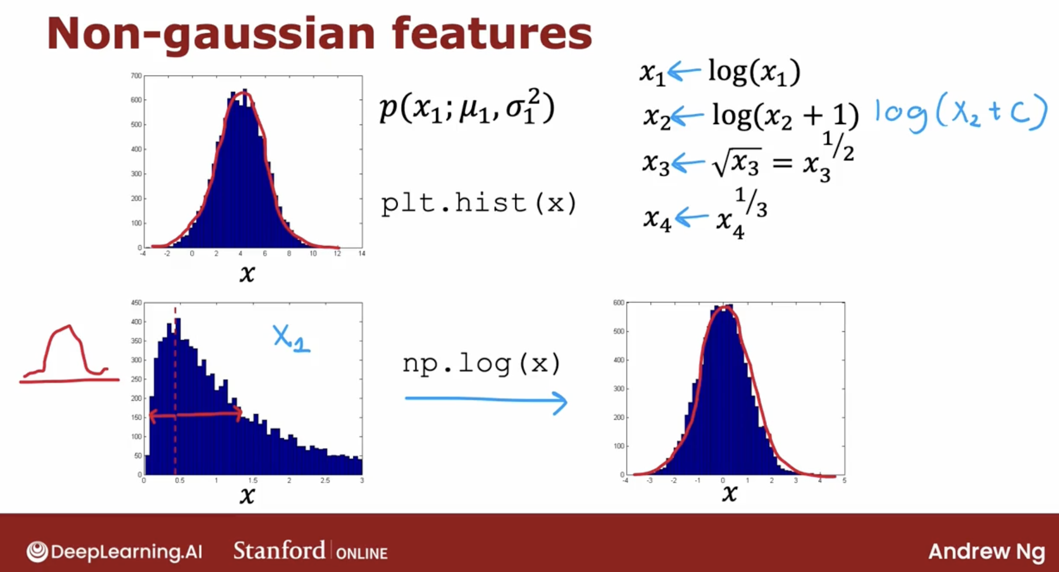
If you read the machine learning literature, there are some ways to automatically measure how close these distributions are to Gaussian. But I found it in practice, it doesn’t make a big difference, if you just try a few values and pick something that looks right to you, that will work well for all practical purposes.
3.5 Anomaly detection vs supervised learning
When you have a few positive examples with y = 1 and a large number of negative examples say y = 0? When should you use anomaly detection and when should you use supervised learning?
The decision is actually quite subtle in some applications.
When you recall that the parameters for p of x are learned only from the negative examples and this much smaller. So the positive examples is only used in your cross validation set and test set for parameter tuning and for evaluation.
3.5.1 key diff
But it turns out that the way anomaly detection looks at the data set versus the way supervised learning looks at the data set are quite different.
Because what anomaly detection does is it looks at the normal examples that is the y = 0 negative examples and just try to model what they look like. And anything that deviates a lot from normal It flags as an anomaly. Including if there’s a brand new way for an aircraft engine to fail that had never been seen before in your data set.
And with supervised learning, we tend to assume that the future positive examples are likely to be similar to the ones in the training set.
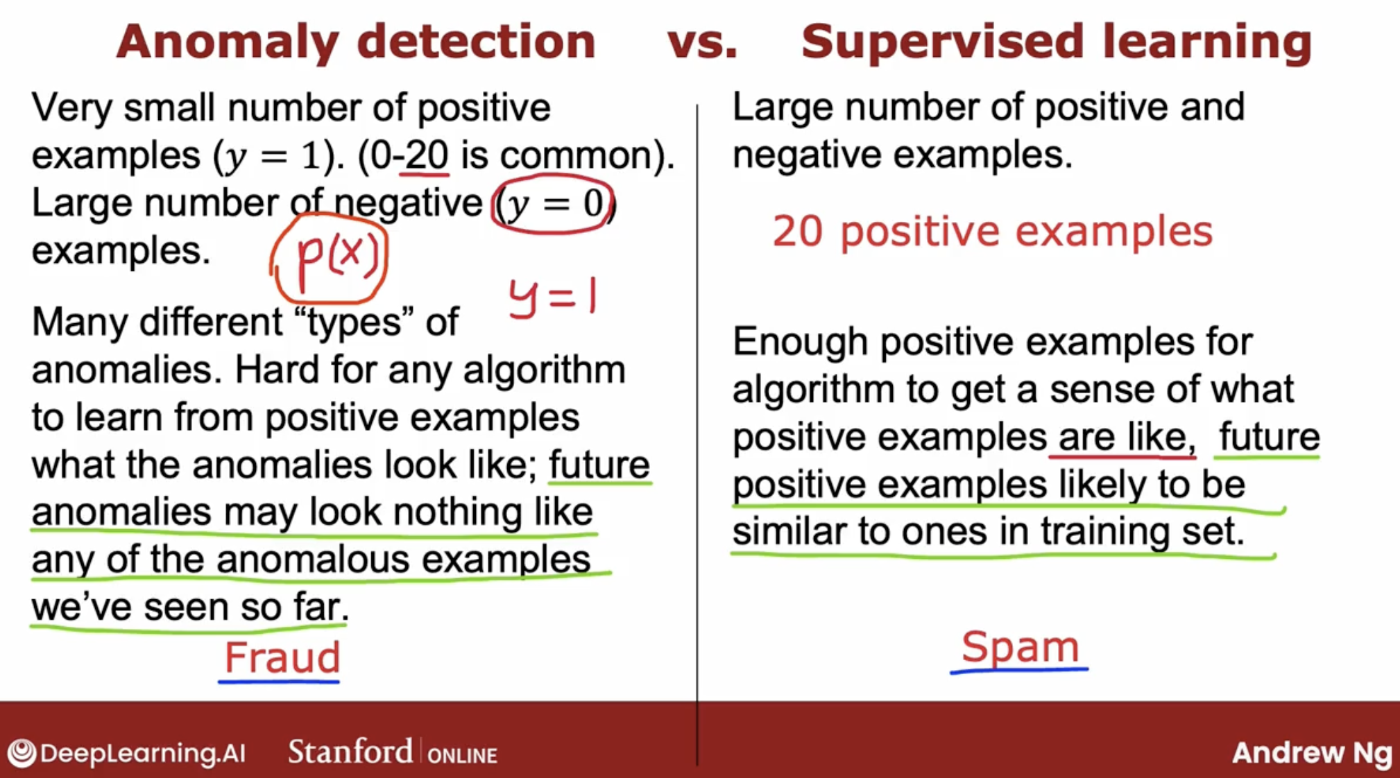
So that’s why supervised learning works well for spam because it’s trying to detect more of the types of spam emails that you have probably seen in the past in your training set.
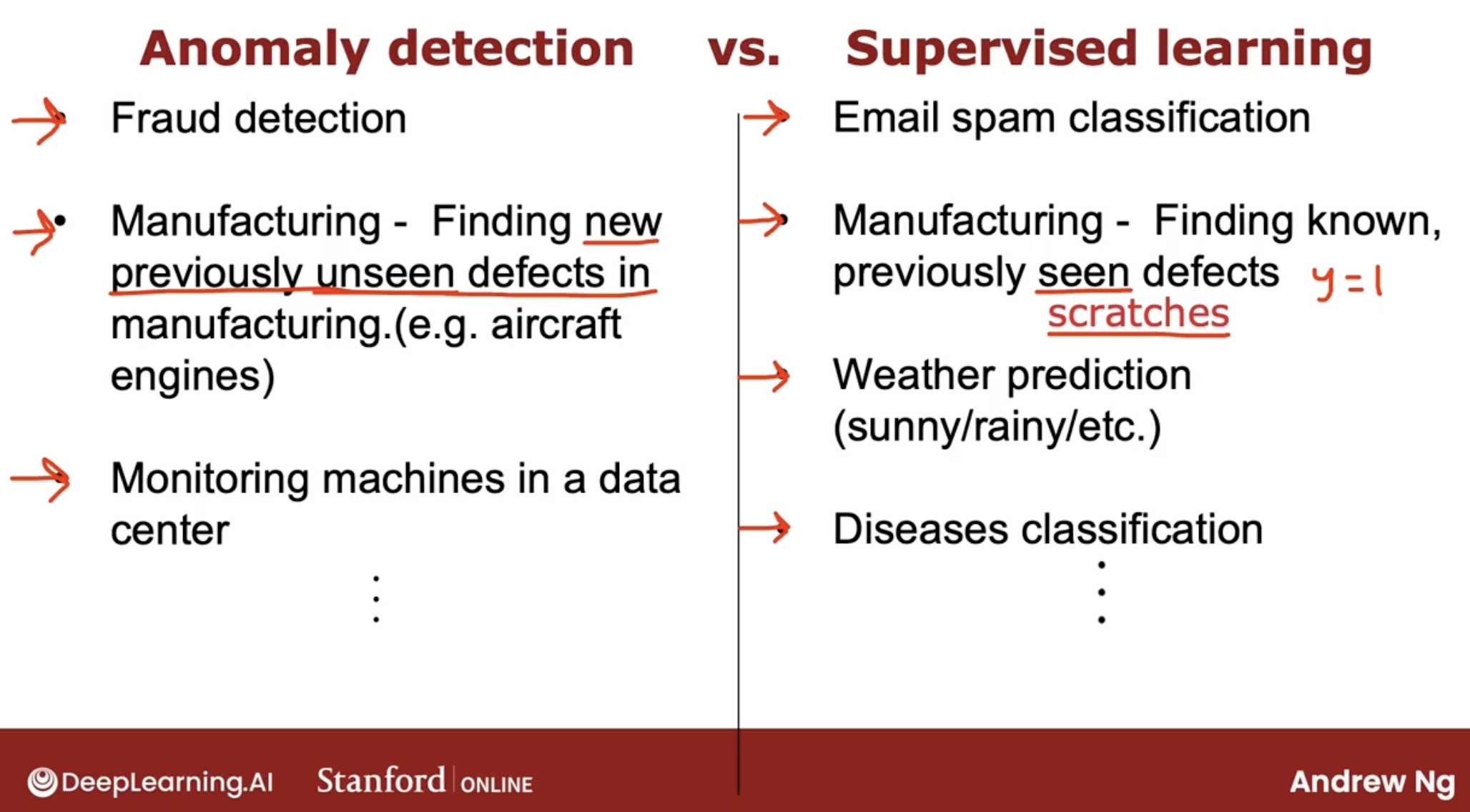
Whereas if you’re trying to detect brand new types of fraud that have never been seen before, then anomaly detection maybe more applicable.
3.5.2 key diff example in manufacturing
supervised learning
- It turns out that the manufacturing supervised learning is also used to find defects. The more for finding known and previously seen defects.
- demo: defect on smartphones
anomaly detection
- Whereas if you suspect that they’re going to be brand new ways for something to go wrong in the future, then anomaly detection will work well.
- demo: monitoring machines in the data center, especially the machine’s been hacked.
3.5.3 about the feature choose
In supervised learning, if you don’t have the features quite right, or if you have a few extra features that are not relevant to the problem, that often turns out to be okay.
Because the algorithm has to supervised signal that is enough labels why for the algorithm to figure out what features ignore, or how to re scale feature and to take the best advantage of the features you do give it.
intuition about unreasonable predict, caused by feature need optimized
When you’ve learned the model P of X from your unlabeled data, the most common problem that you may run into is that, P of X is comparable in value say is, large for both normal and for anomalous examples.
This is obviously a problem. So the algorithm will fail to flag this particular example as an anomaly.
In that case, what I would normally do is, try to look at that example and try to figure out what is it that made me think is an anomaly, even if this feature X one took on values similar to other training examples.
And if I can identify some new feature say X two, that helps distinguish this example from the normal examples. Then adding that feature, can help improve the performance of the algorithm.
So just to summarize the development process will often go through is, to train the model and then to see what anomalies in the cross validation set the algorithm is failing to detect. And then to look at those examples to see if that can inspire the creation of new features that would allow the algorithm to spot.
That example takes on unusually large or unusually small values on the new features, so that you can now successfully flag those examples as anomalies.
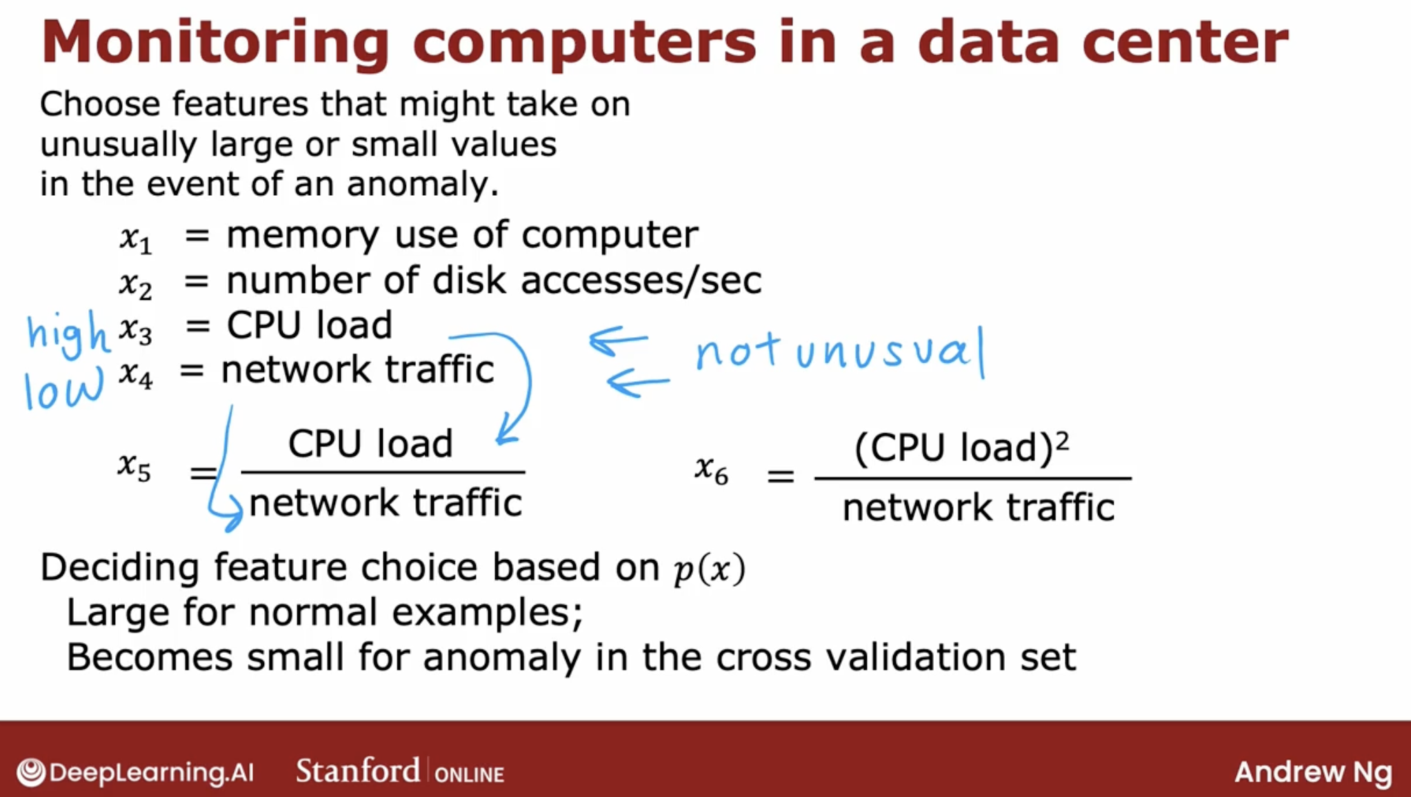
And you can play around with different choices of these features. In order to try to get it so that P of X is still large for the normal examples but it becomes small in the anomalies in your cross validation set.
3.5.4 summary
- Anomaly detection tries to find brand new positive examples that may be unlike anything you’ve seen before.
- Where supervised learning looks at your positive examples and tries to decide if a future example is similar to the positive examples that you’ve already seen.