【Meachine Learning】08 Neural Network

1 simple history

1.1 simple history timeline

So neural networks has started with the motivation of trying to build software to mimic the brain.

Work in neural networks had started back in the 1950s, and then it fell out of favor for a while.

Then in the 1980s and early 1990s, they gained in popularity again and showed tremendous traction in some applications like handwritten digit recognition, which were used even backed then to read postal codes for writing mail and for reading dollar figures in handwritten checks. But then it fell out of favor again in the late 1990s.

It was from about 2005 that it enjoyed a resurgence and also became re-branded little bit with deep learning. One of the things that surprised me back then was deep learning and neural networks meant very similar things. But maybe under-appreciated at the time that the term deep learning, just sounds much better because it’s deep and this learning. So that turned out to be the brand that took off in the last decade or decade and a half.

Since then, neural networks have revolutionized application area after application area.

• first, speech recognition
• then, computer visionSometimes people still speak of the ImageNet moments in 2012
• Then the next few years, it made us inroads into texts or into natural language processing
• and so on and so forth.

Now, neural networks are used in everything from climate change to medical imaging to online advertising to prouduct recommendations and really lots of application areas of machine learning now use neural networks.

Even though today’s neural networks have almost nothing to do with how the brain learns, there was the early motivation of trying to build software to mimic the brain.

some other info:

• why ai take off now

1.2 simple summary

When neural networks were first invented many decades ago, the original motivation was to write software that could mimic how the human brain or how the biological brain learns and thinks.

Even though today, neural networks, sometimes also called artificial neural networks, have become very different than how any of us might think about how the brain actually works and learns.

Some of the biological motivations still remain in the way we think about artificial neural networks or computer neural networks today.

2 simple intuition

2.1 intuition by biology and artificial neural network

So how does the brain work?

let’s analogy the two neuron.

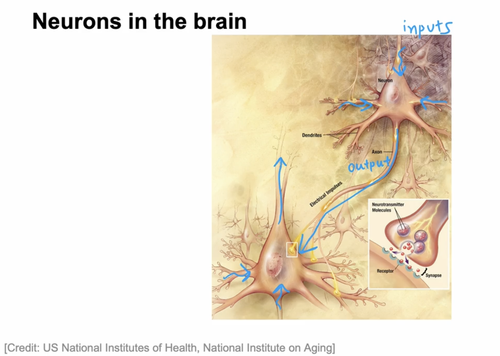
As we saw on the previous slide, the neuron has different inputs.

biological neuron

• In a biological neuron, the input wires are called the dendrites, and it then occasionally sends electrical impulses to other neurons via the output wire, which is called the axon.
• Don’t worry about these biological terms. If you saw them in a biology class, you may remember them, but you don’t really need to memorize any of these terms for the purpose of building artificial neural networks.
• And this biological neuron may then send electrical impulses that become the input to another neuron.

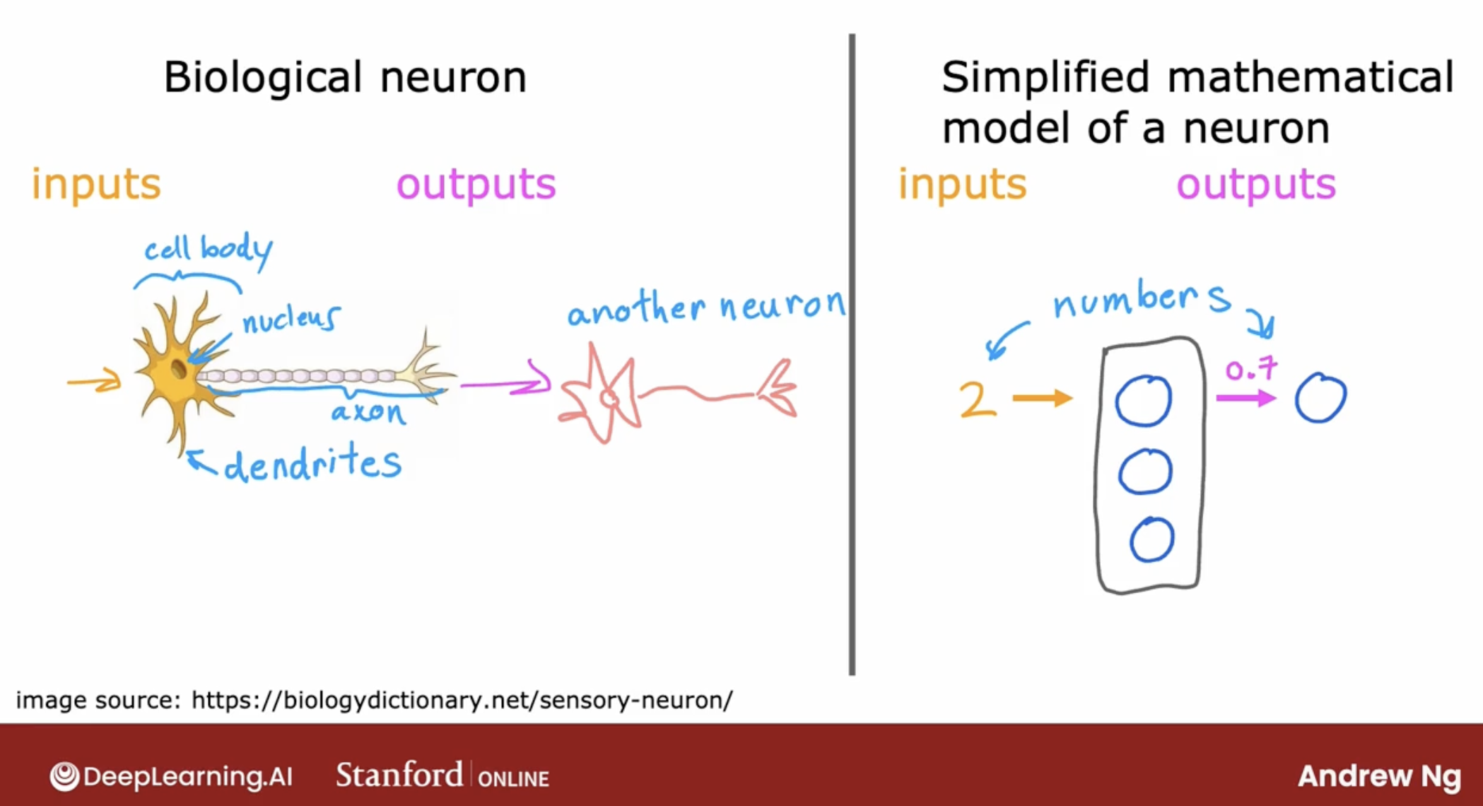
artificial neuron

• So the artificial neural network uses a very simplified Mathematical model of what a biological neuron does.
• I’m going to draw a little circle here to denote a single neuron. What a neuron does is it takes some inputs, one or more inputs, which are just numbers. It does some computation and it outputs some other number, which then could be an input to a second neuron, shown here on the right.
• When you’re building an artificial neural network or deep learning algorithm, rather than building one neuron at a time, you often want to simulate many such neurons at the same time.
• In this diagram, I’m drawing three neurons. What these neurons do collectively is input a few numbers, carry out some computation, and output some other numbers.

caveat:

• even though I made a loose analogy between biological neurons and artificial neurons, I think that today we have almost no idea how the human brain works.
• So as you go deeper into neural networks and into deep learning, even though the origins were biologically motivated, don’t take the biological motivation too seriously.
• In fact, those of us that do research in deep learning have shifted away from looking to biological motivation that much.

2.2 intuition by demo: demand prediction with one neuron

First, illustrate neuron concept by demand prediction with one neuron.

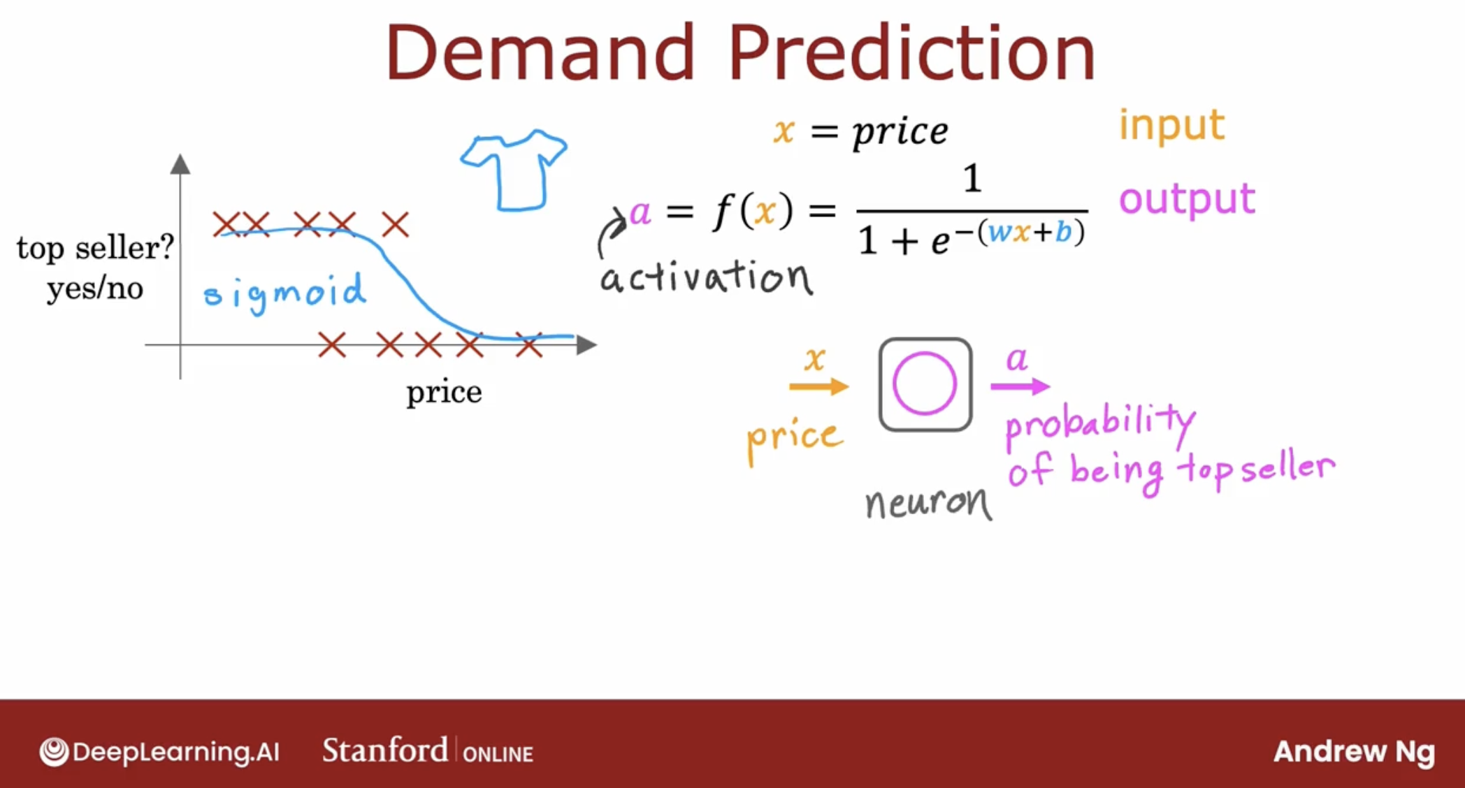
As we can see, this one neuron only do one thing:

• input the price of the product
• use the logistic regression to predict the demand of the product.
• output the probability of this product will be top seller.

So, this is a simple neuron.

2.3 intuition by demo: demand prediction with multiple neurons

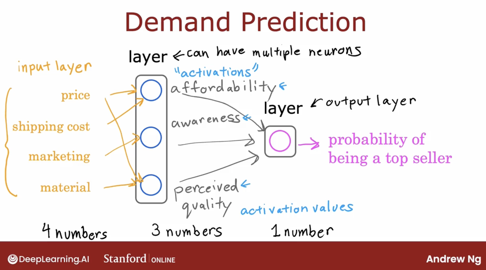
Let’s take a look at the multiple neurons.

• let’s say we have 4 featrues: price, shipping cost, marketing, material.
• and 3 neurons: affordability, awareness, perceived quality.
• and these 3 neurons will output the probability of the product will be top seller.
• affordability is dependent on price and shipping cost, awareness is dependent on marketing and material, perceived quality is dependent on price, material.
• and the probability of the product will be top seller is the weighted sum of these 3 neurons.

output of every one neuron is called activation, and the activation function is called activation function.

activation function is a function that takes the weighted sum of the inputs and returns a single number. activation function can be linear, sigmoid, etc.

And, if we say every neuron can have some relationship with every neural in the previous layer, then we can connect every neuron in the hidden layer with every neuron in the input layer, and, we can use: vectorized computation, it looks like what we saw in the previous blog.

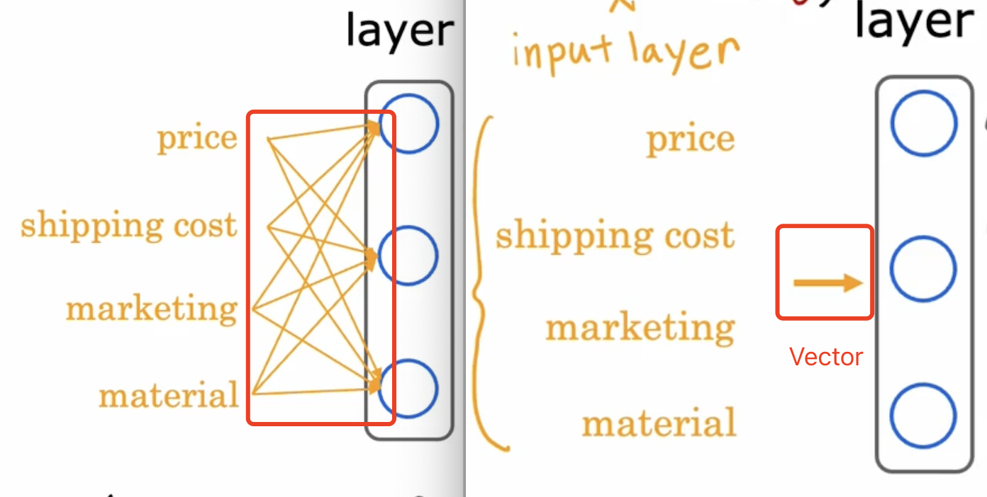
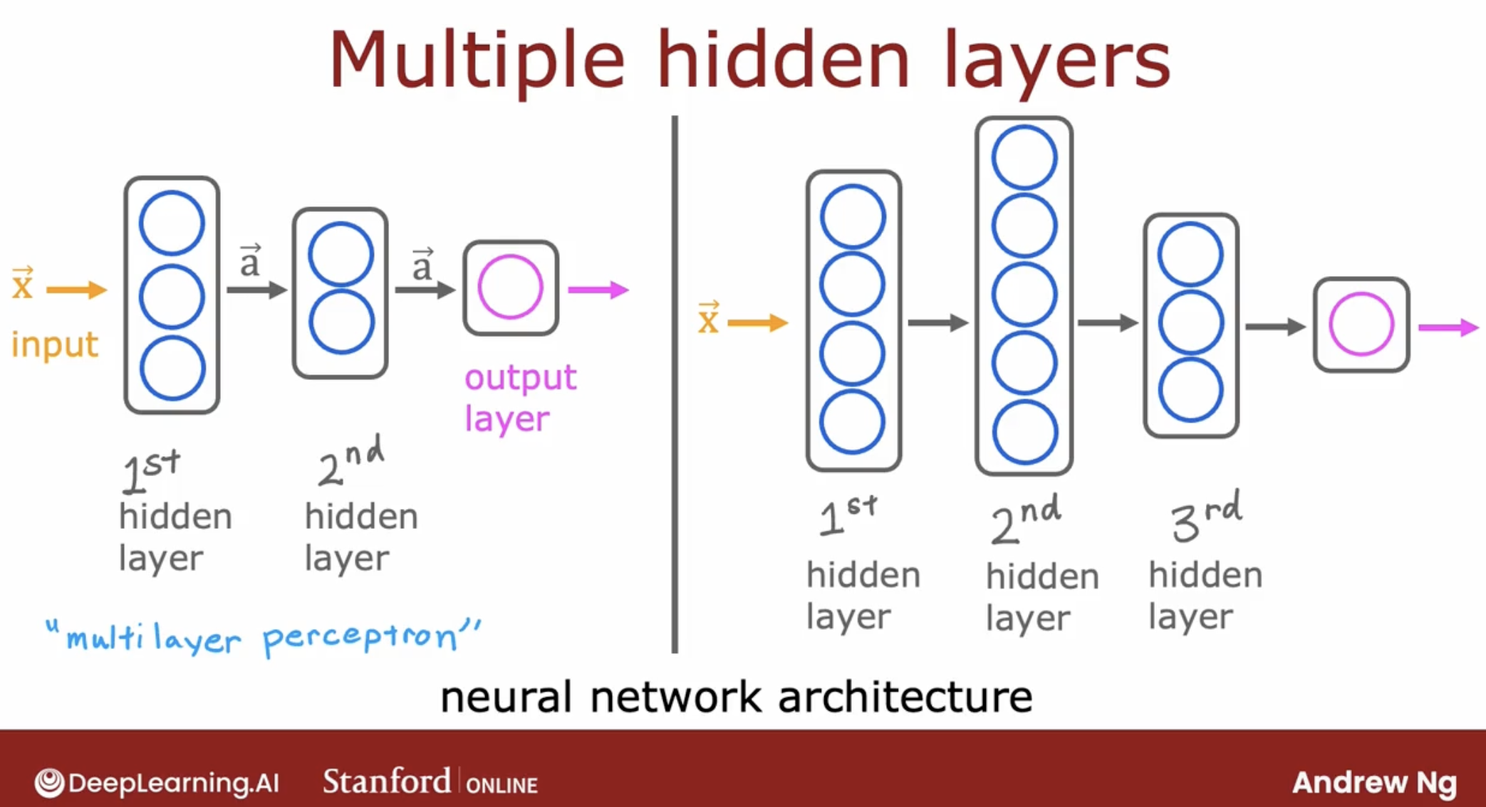
So, this is a multiple neurons. and all the input featuers are called input layer, the output is called output layer, all the layers in between are called hidden layer.

hidden layer can be more than one.

One note, even though I previously described this neural network as computing affordability, awareness, and perceived quality, one of these really nice properties of a neural network is when you train it from data, you don’t need to go in to explicitly decide what other features, such as affordability and so on, that the neural network should compute instead or figure out all by itself what are the features it wants to use in this hidden layer.

That’s what makes it such a powerful learning algorithm.

some terminology

• multilayer perceptron, is same as neural network with multiple hidden layers.

2.4 intuition by demo: face recognition

So, let’s take a look at the face recognition.

let’s say one image is 1000x1000 pixels, if the image is black and white, then every pixel can be represented by one number, and the total number of pixels is 1000x1000=1,000,000.

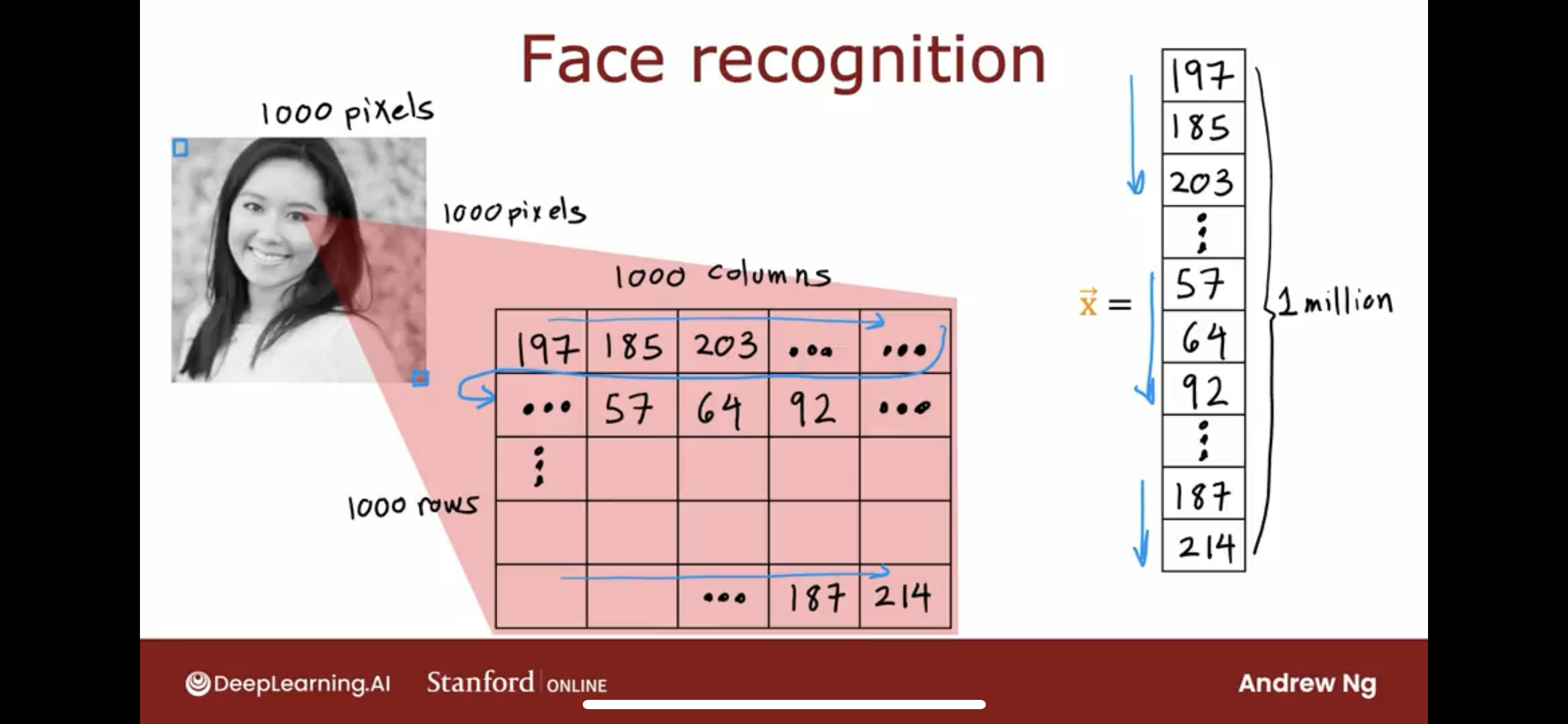
and we store the 1 million numbers in a vector as the input layer.

and we can use a neural network to predict the probability of this image is a certain person.

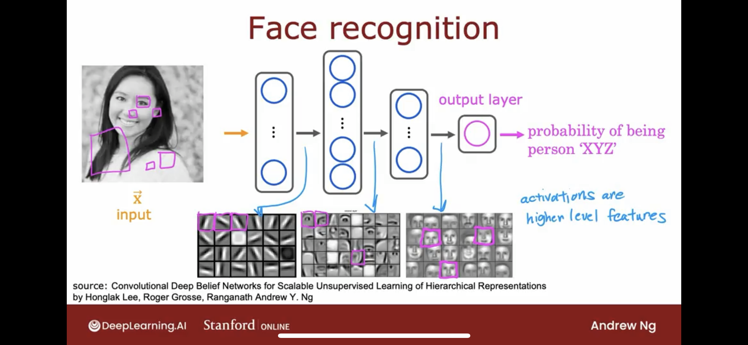
It turns out that when you train a system like this on a lot of pictures of faces and you peer at the different neurons in the hidden layers to figure out what they may be computing this is what you might find.

• In the first hidden layer, you might find one neuron that is looking for the low vertical line or a vertical edge like that.
• A second neuron looking for a oriented line ororiented edge like that.
• The third neuron looking for a line at that orientation
• and so on.

In the earliest layers of a neural network, you might find that the neurons are looking for very short lines or very short edges in the image.

If you look at the next hidden layer, you find that these neurons might learn to group together lots of little short lines and little short edge segments in order to look for parts of faces.

For example, each of these little square boxes is a visualization of what that neuron is trying to detect.

• This first neuron looks like it’s trying to detect the presence or absence of an eye in a certain position of the image.
• The second neuron, looks like it’s trying to detect like a corner of a nose and maybe this neuron over here is trying to detect the bottom of an ear.
• Then as you look at the next hidden layer in this example, the neural network is aggregating different parts of faces to then try to detect presence or absence of larger, coarser face shapes.
• Then finally, detecting how much the face corresponds to different face shapes creates a rich set of featuresthat then helps the output layer try to determine the identity of the person picture.

So, we can see, activations are higher level features.

A remarkable thing about the neural network is you can learn these feature detectors at the different hidden layers all by itself.

2.5 intuition by demo: car recognition

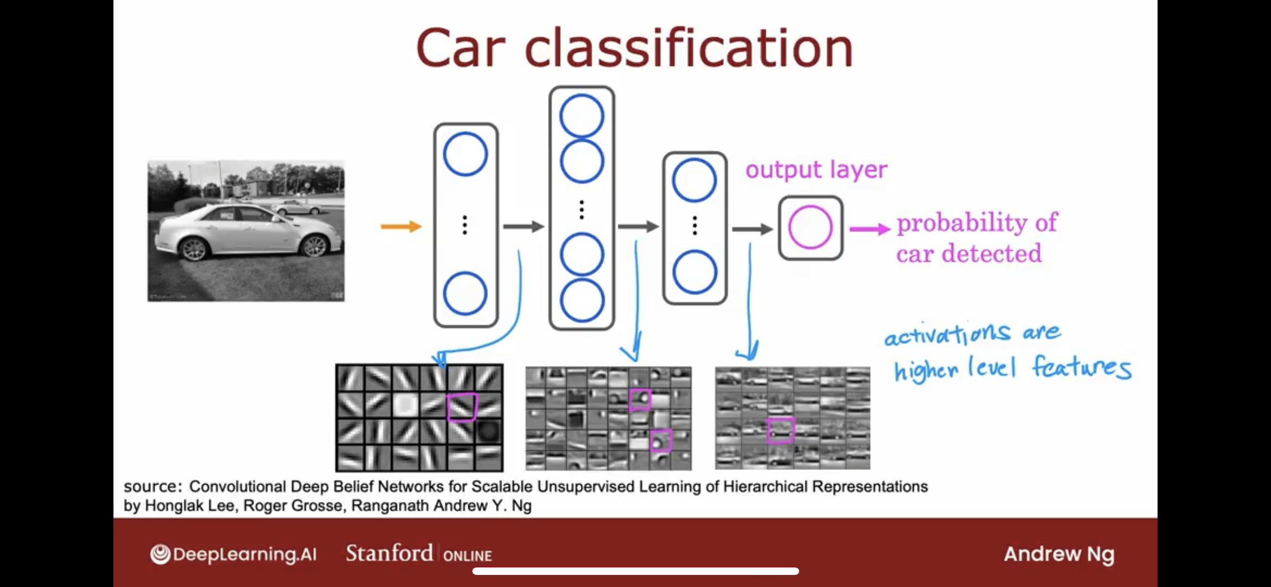
same as face recognition:

• digit the image into a vector.
• create multiple hidden layers, every neuron in the hidden layer is looking for a different feature.
• and the output layer is trying to predict the probability of the image is a certain car.

Again, the neural network is able to learn these feature detectors at the different hidden layers all by itself.

2.6 intuition by hidden layers detail

layer 1

let’s take a look at layer 1.

Note: layer 0 is the input layer.

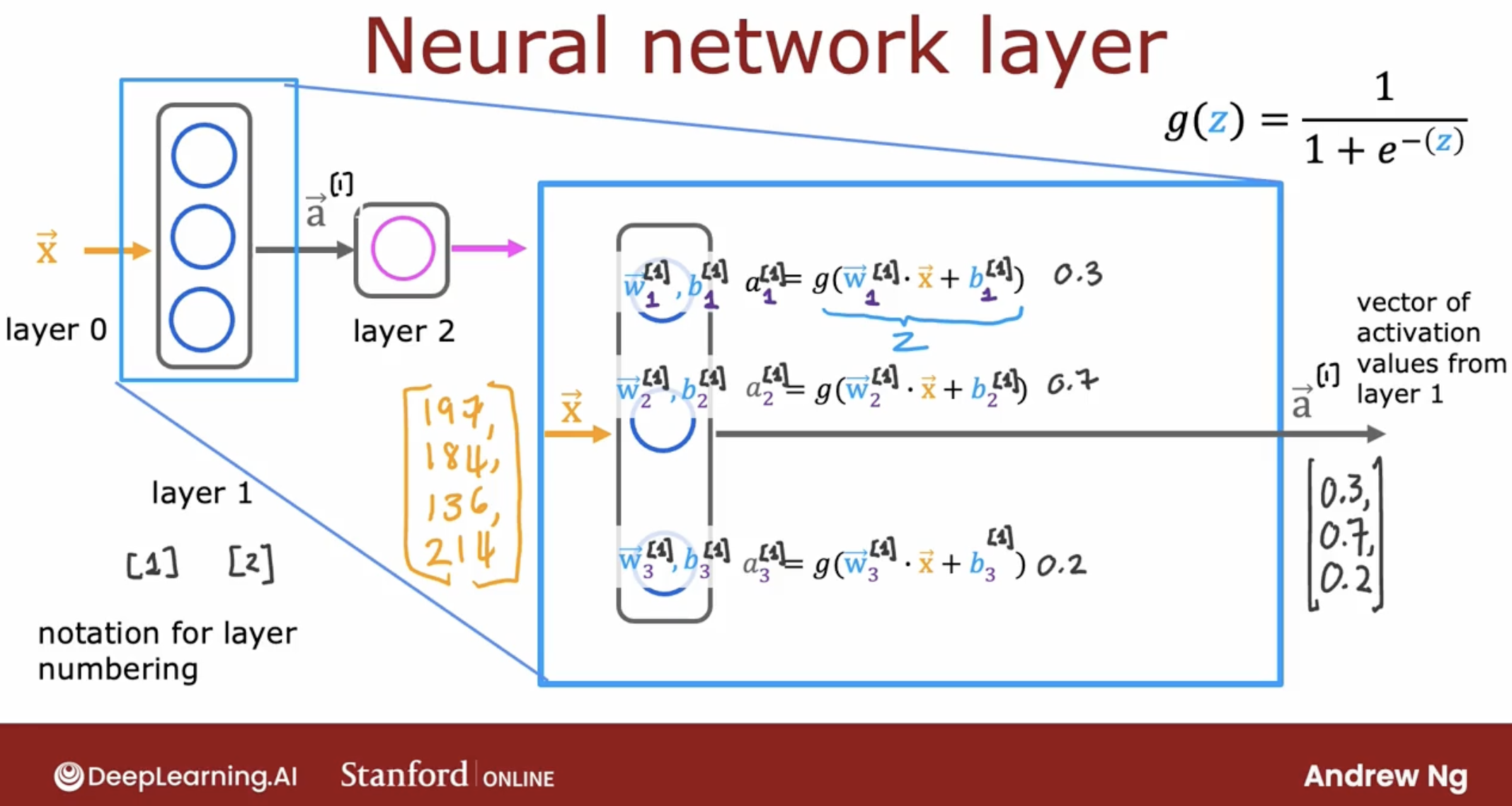
As we can see, the three neurons in the layer 1 are all sigmoid neurons, because the activation function of neuron is sigmoid function. Of course, the activation function of neuron can not only be sigmoid function, but also be linear function, etc.

Note: we can use different activation function for different neuron in the hidden layer.

layer 2

Let’s take a look at the layer 2.

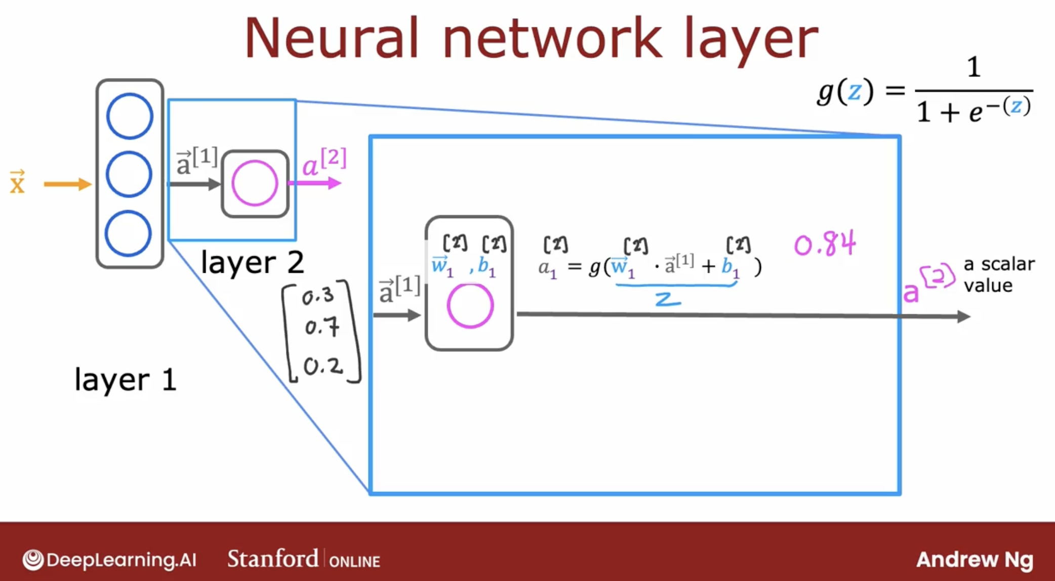
As we can see, the one neuron in the layer 2 is a sigmoid neuron.

Althrough layer 2 is the output layer, but it’s output is a vector, not a number.

So we need to handle the vector.

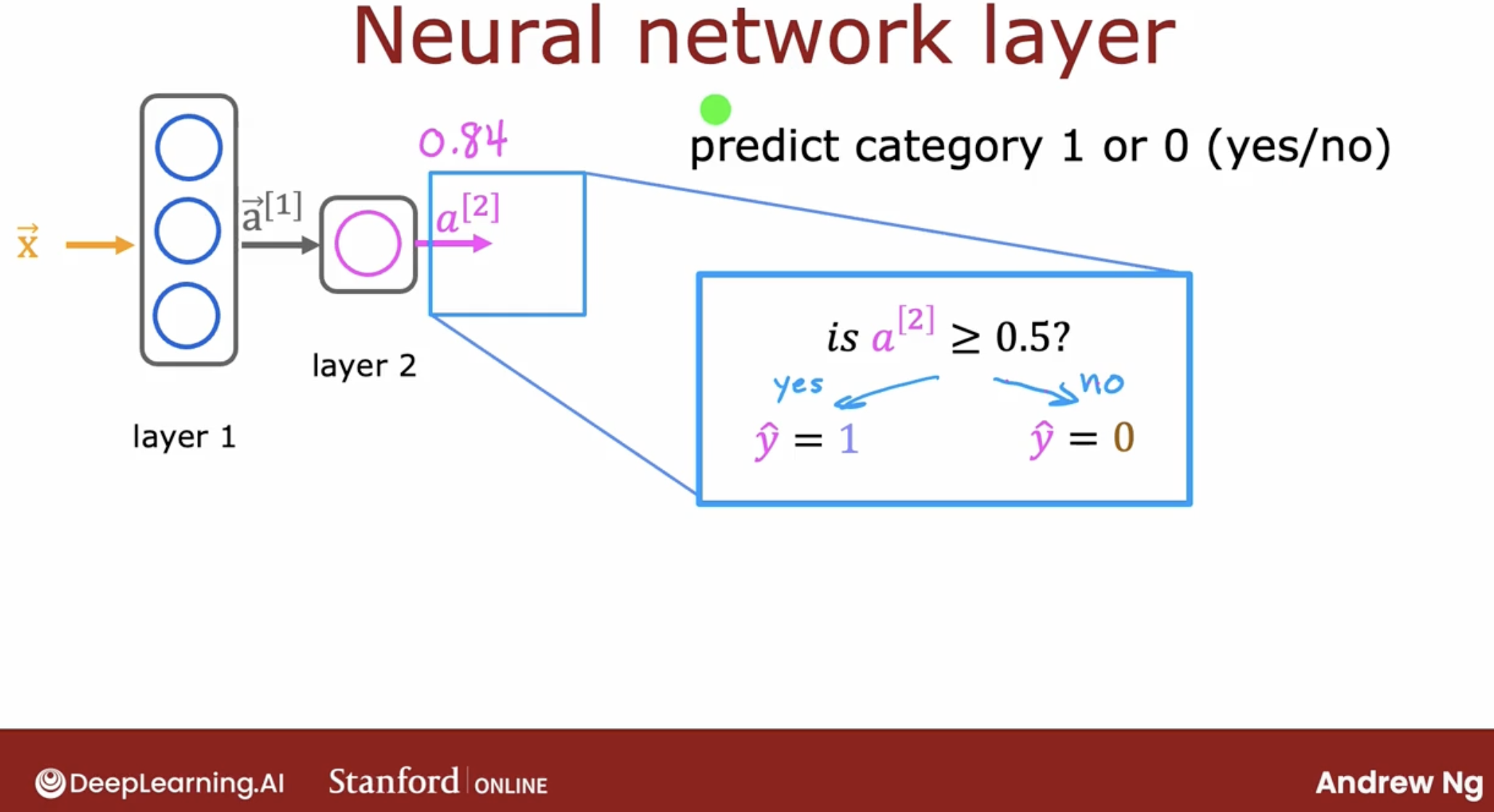
Then, we can get the result 0 or 1.

2.7 intuition summary

So, let’s summarize the intuition of neural network.

3 inference

3.1 inference intuition

Let’s take what we’ve learned and put it together into an algorithm to let your neural network make inferences or make predictions.

This will be an algorithm called forward propagation.

inference, using the forward propagation algorithm.

forward propagation algorithm: let your neural network make inferences or make predictions.

Because this computation goes from left to right, you start from x and compute a1, then a2, then a3. This album is also called forward propagation because you’re propagating the activations of the neurons. So you’re making these computations in the forward direction from left to right.

And by the way, this type of neural network architecture where you have more hidden units initially and then the number of hidden units decreases as you get closer to the output layer. There’s also a pretty typical choice when choosing neural network architectures.

3.2 inference fake code

let’s take a look at the code.

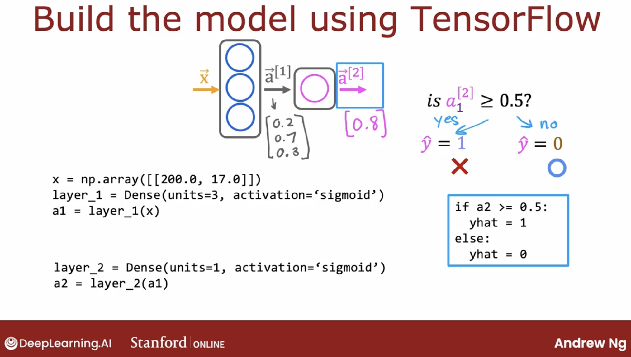
• layer 0 is input layer. denoted by $\mathbf{x}$
• layer 1 has 3 neurons, suppose all activation function are sigmoid function.
  • Dense: dense means every neuron in the current layer is connected to every neuron in the previous layer.
• layer 2 has 1 neuron, suppose activation function is sigmoid function.

Note: every layer output is a vector.

So summary, there are 5 steps to build a neural network:

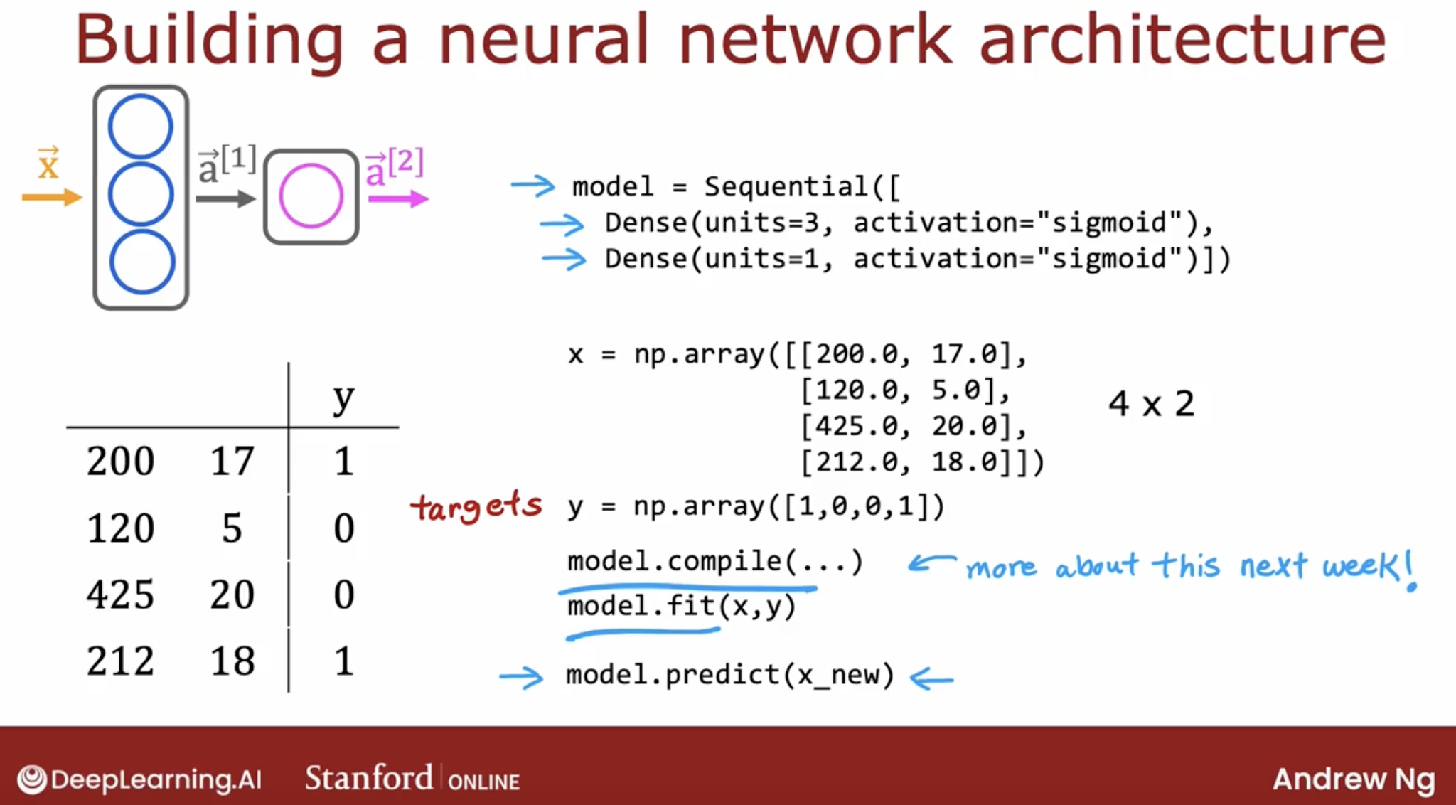
1. Define the network structure.
   • use tf.keras.Sequential and tf.keras.layers.Dense to define the network structure.
2. define the network
   • loss function.
   • optimizer.
   • and so on.
3. define the X and Y.
4. train the network.
   • use model.fit to train the network.
5. evaluate the network.
   • use model.evaluate to evaluate the network.

3.3 intuition about the dense layer

First, let’s see the every neuron do what.

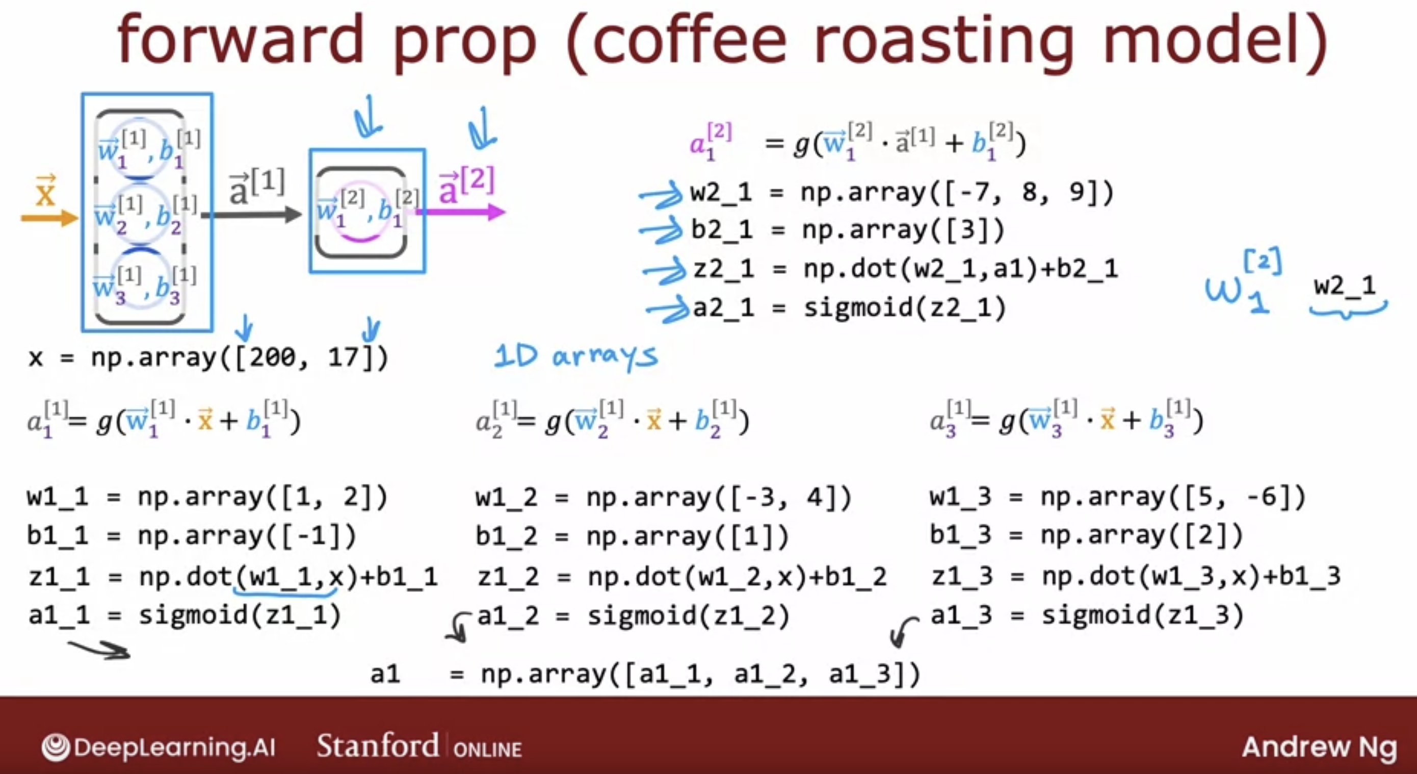
Then, let’s see the whole network with numpy, to understand the dense layer.

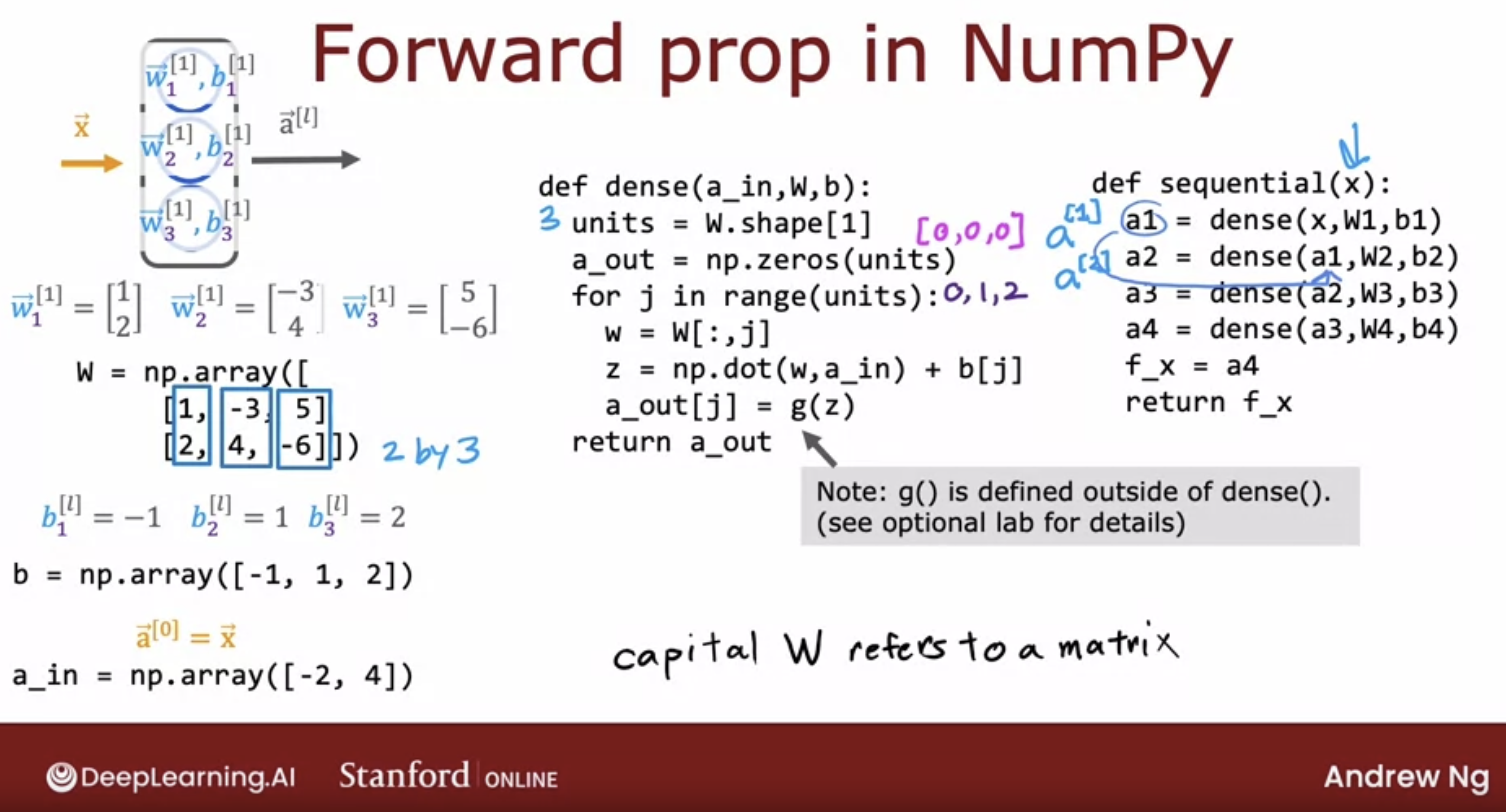
more doc:

• more about numpy operation

3.4 code demo: output layer has one neuron

3.4.1 code

binary_handwritten_digit_recognization

3.4.2 code instructions

So, that’s how you can train a neural network in TensorFlow.

• Step 1 is to specify the model, which tells TensorFlow how to compute for the inference.
• Step 2 compiles the model using a specific loss function.
• Step 3 is to train the model.

and these steps are the similar to the model we learned before, just like the logistic regression.

about cost function

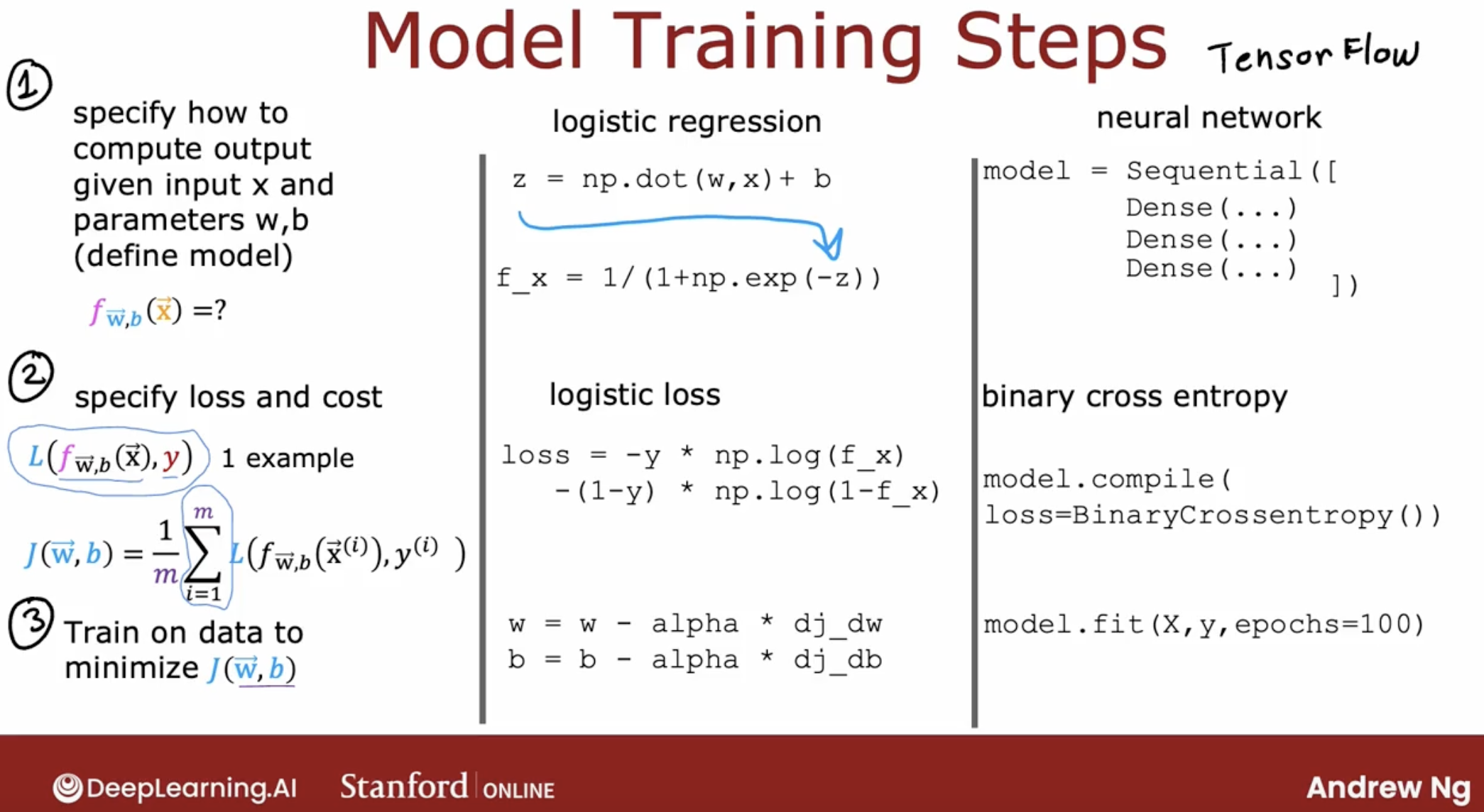
• binary cross entropy: same as logistic regression loss function before, classification problem
• mean squared error: usually in regression problem.

more doc:

• more cost function

3.5 about use library

In order to use gradient descent, the key thing you need to compute is these partial derivative terms. What TensorFlow does, and, in fact, what is standard in neural network training, is to use an algorithm called backpropagation in order to compute these partial derivative terms. TensorFlow can do all of these things for you.

One pattern I’ve seen across multiple ideas is as the technology evolves, libraries become more mature, and most engineers will use libraries rather than implement code from scratch. There have been many other examples of this in the history of computing.

But today, deep learning libraries have matured enough that most developers will use these libraries, and, in fact, most commercial implementations of neural networks today use a library like TensorFlow or PyTorch.

But as I’ve mentioned, it’s still useful to understand how they work under the hood so that if something unexpected happens, which still does with today’s libraries, you have a better chance of knowing how to fix it.

3.6 about the activation function

The most common activation functions are the following:

activation function	function
linear	$f(z) = z$
sigmoid	$f(z) = \frac{1}{1+e^{-z}}$
relu()	rectified linear unit(ReLU) $f(z) = max(0,z)$

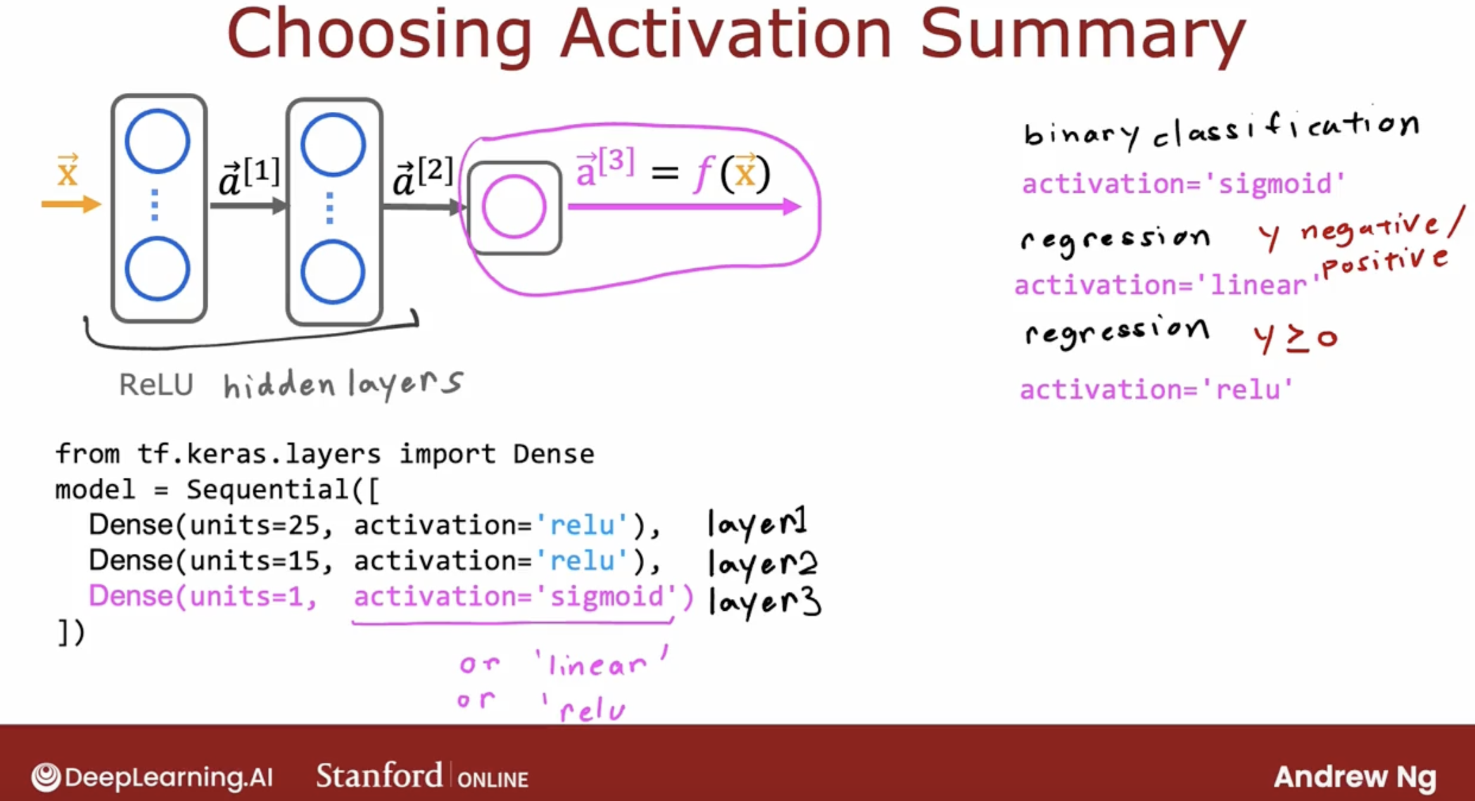
Here is the different activation functions intuition.

And, here is how to choose the activation function.

activation function	applicable scenario
sigmoid	binary classification
linear	y is continuous, positive or negative
relu()	y >= 0

By the way, if you look at the research literature, you sometimes hear of authors using even other activation functions, such as the tan h activation function or the LeakyReLU activation function or the swish activation function. Every few years, researchers sometimes come up with another interesting activation function, and sometimes they do work a little bit better.

But I think for the most part, and for the vast majority of applications what you learned about in this video would be good enough.

3.7 code demo: output layer has multiple neurons

3.7.1 code instructions

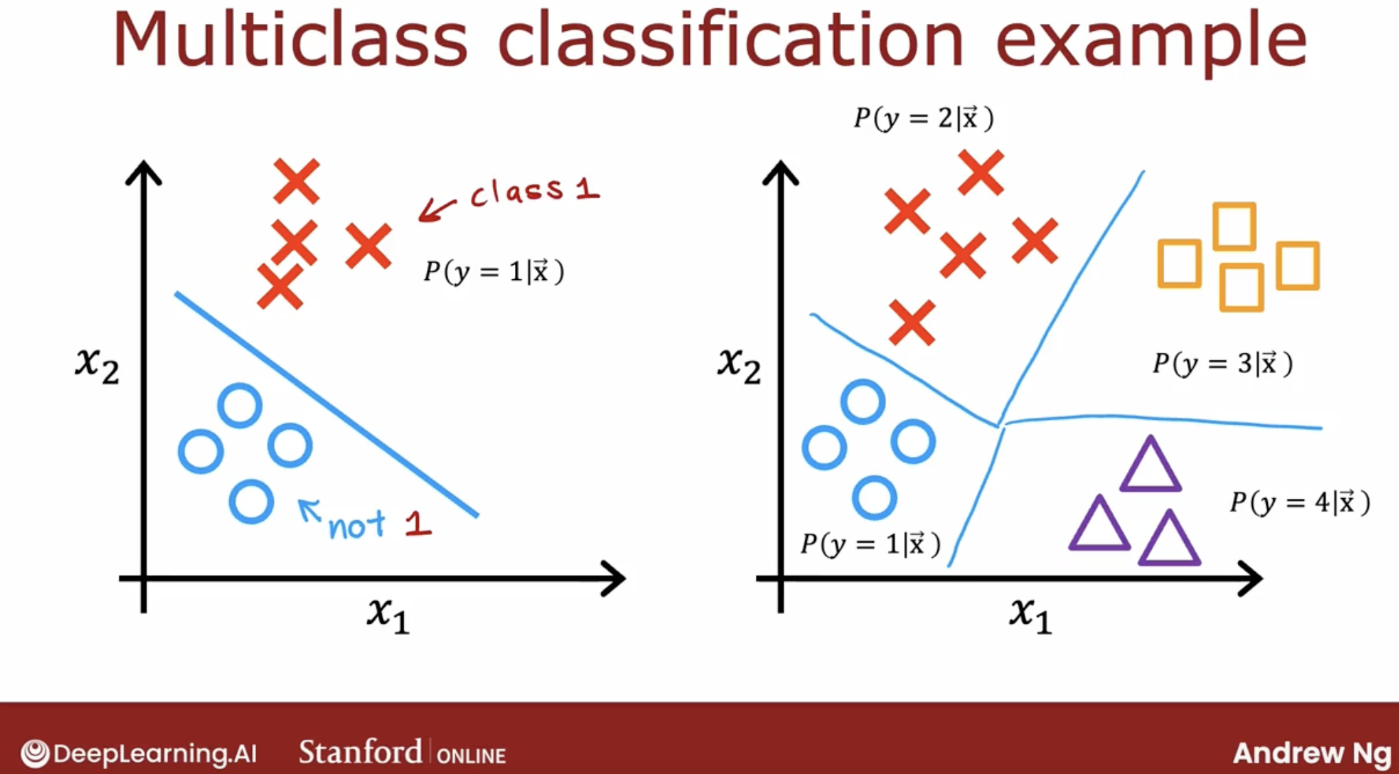
3.7.1.1 problem intuition

Let’s take a look what this problem looks like.

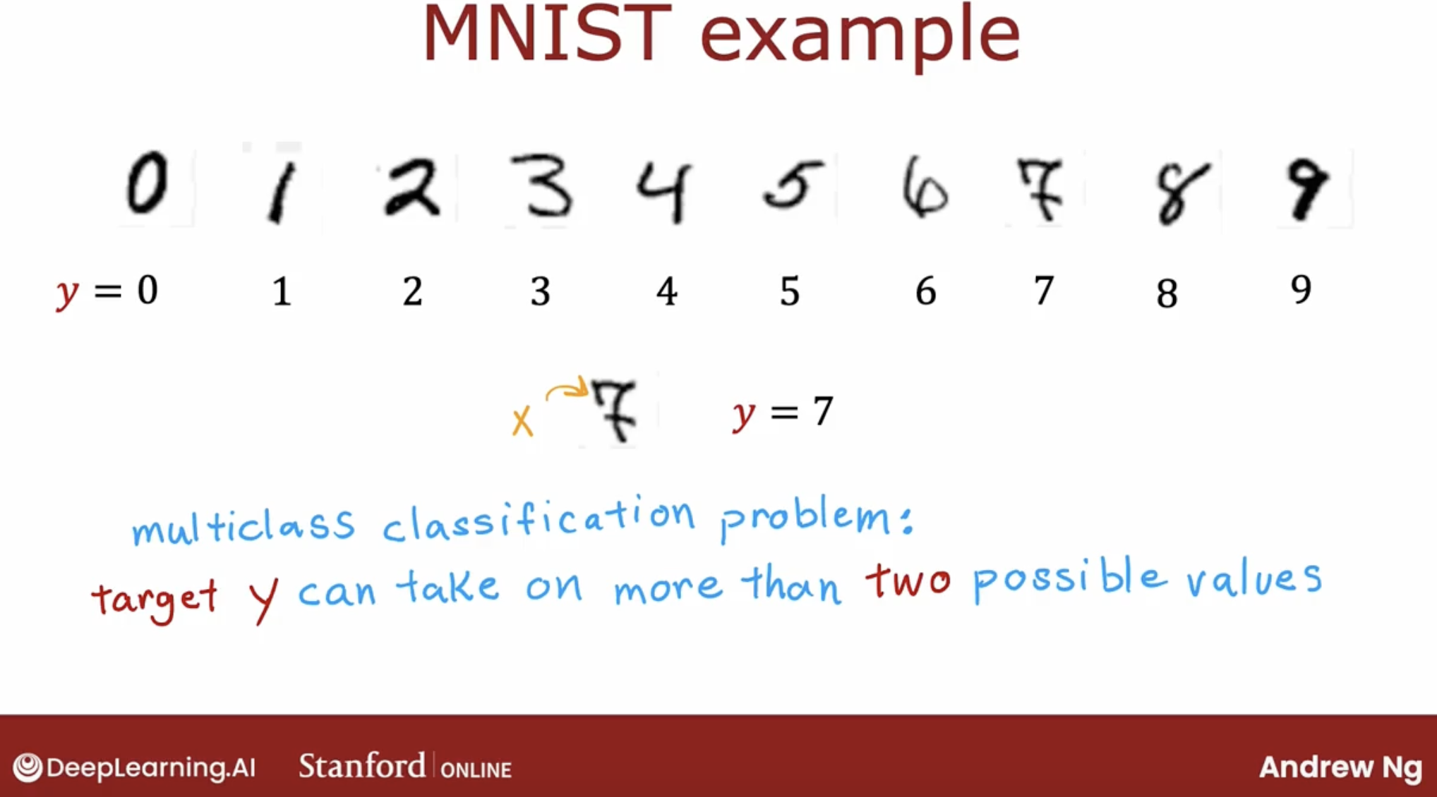
And, this is also the classification problem, but not only two classes, but multiple classes.

3.7.1.2 softmax intuition

So, how can we calculate the probability of each class?

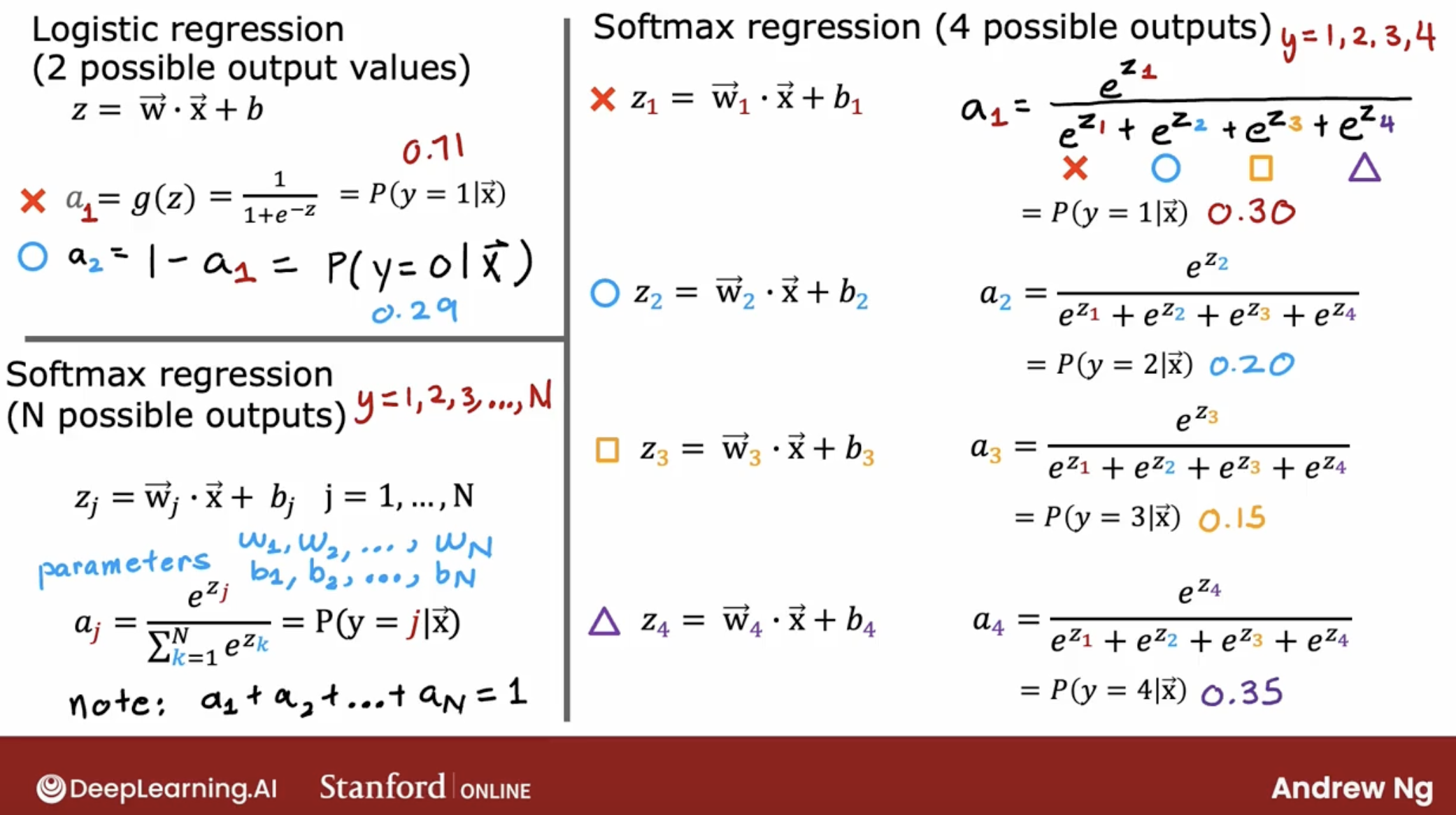
We say if class number is 2, then probability of:

• class 1: $a_1 = g(z) = \frac{1}{1+ e^{-z}}$
• class 2: $a_2 = 1 - a_1$

When class number is multiple, then the sum of all the probabilities, we say, 1.

\(a_j = \frac{e^{z_j}}{ \sum_{k=1}^{N}{e^{z_k} }} \tag{1}\) The output $\mathbf{a}$ is a vector of length N, so for softmax regression, you could also write: \(\begin{align} \mathbf{a}(x) = \begin{bmatrix} P(y = 1 | \mathbf{x}; \mathbf{w},b) \\ \vdots \\ P(y = N | \mathbf{x}; \mathbf{w},b) \end{bmatrix} = \frac{1}{ \sum_{k=1}^{N}{e^{z_k} }} \begin{bmatrix} e^{z_1} \\ \vdots \\ e^{z_{N}} \\ \end{bmatrix} \end{align}\)

So, here is the intuition of the softmax regression.

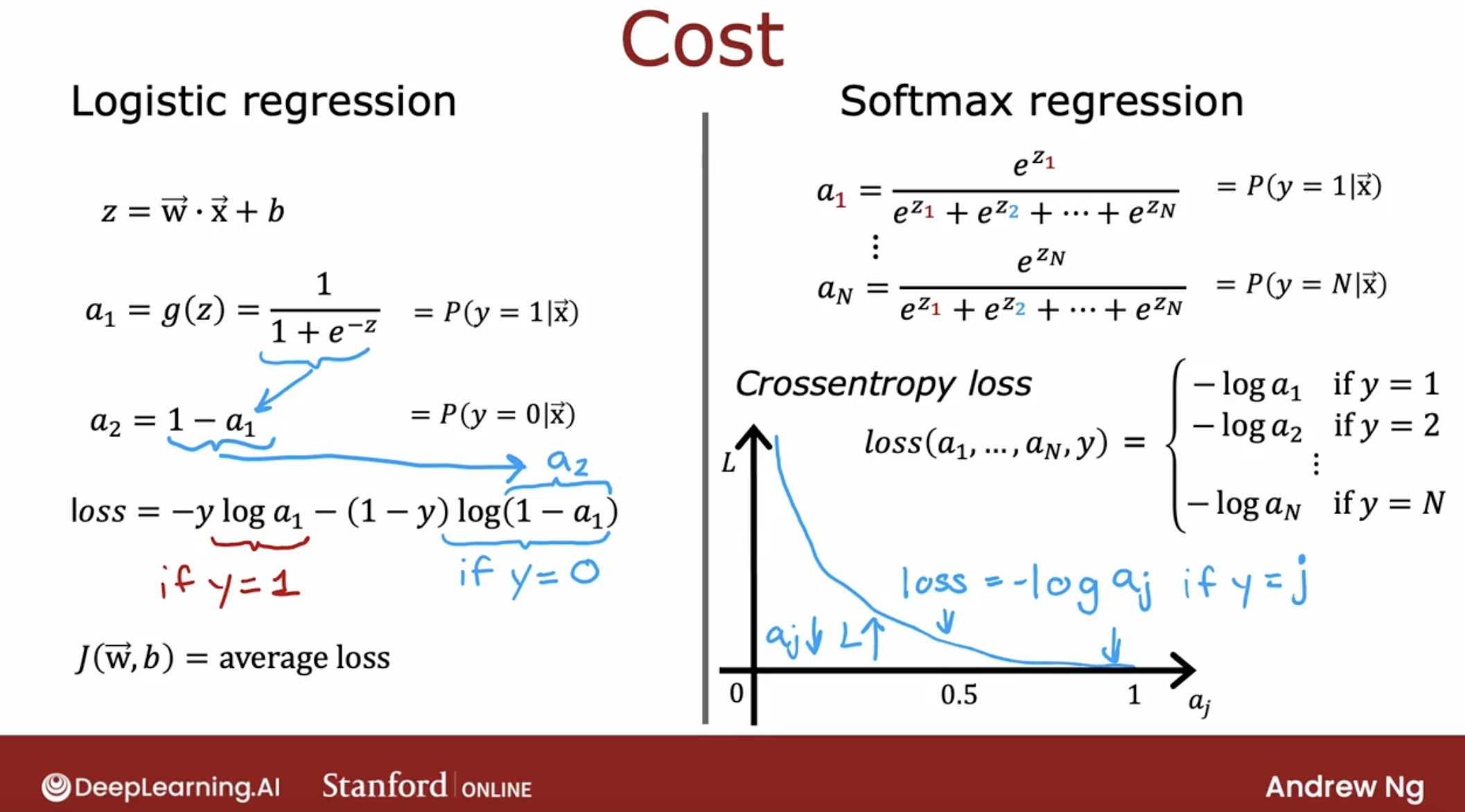
3.7.1.3 softmax regression loss and cost function

And, this is the cross-entropy loss.

\[\begin{equation} L(\mathbf{a},y)=\begin{cases} -log(a_1), & \text{if $y=1$}.\\ &\vdots\\ -log(a_N), & \text{if $y=N$} \end{cases} \end{equation}\]

Now the cost is: \(\begin{align} J(\mathbf{w},b) = -\frac{1}{m} \left[ \sum_{i=1}^{m} \sum_{j=1}^{N} 1\left\{y^{(i)} == j\right\} \log \frac{e^{z^{(i)}_j}}{\sum_{k=1}^N e^{z^{(i)}_k} }\right] \end{align}\)

Where $m$ is the number of examples, $N$ is the number of outputs. This is the average of all the losses.

3.7.1.4 fake code intuition

And, in neural network, different neurons in output layer are independent, let’s how to denote these probabilities.

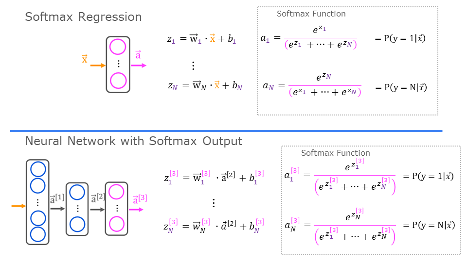
And, here is the fake code.

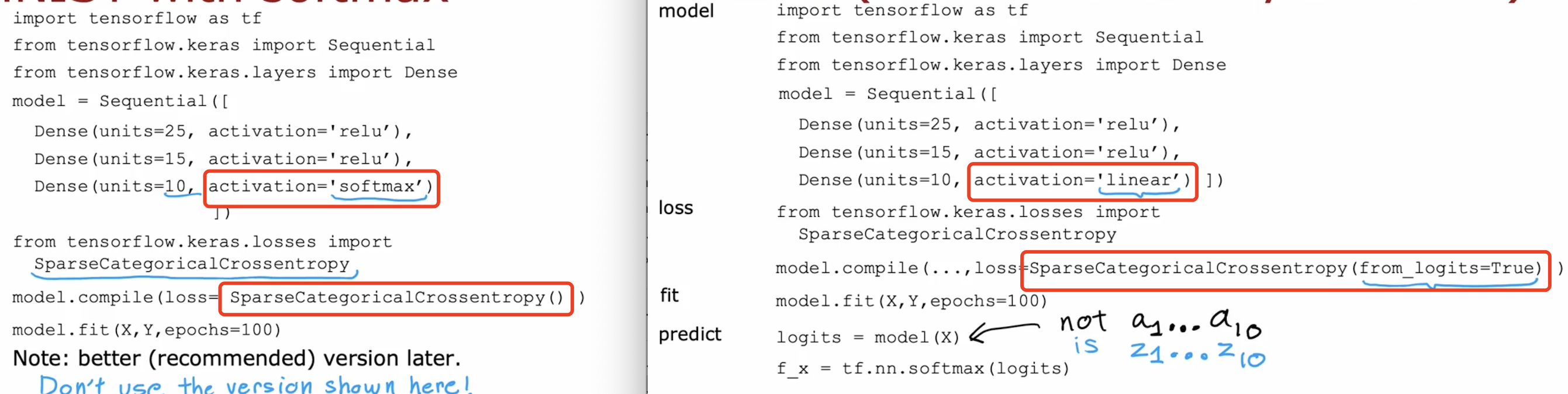
3.7.1.5 optimization: numerical accuracy

And more, we need optimize the fake code.

why? because the numerical accuracy is not good. Here is the reason.

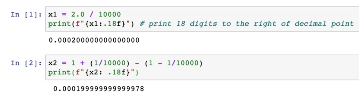
So, how to optimize the numerical accuracy?

1. about logistic regression

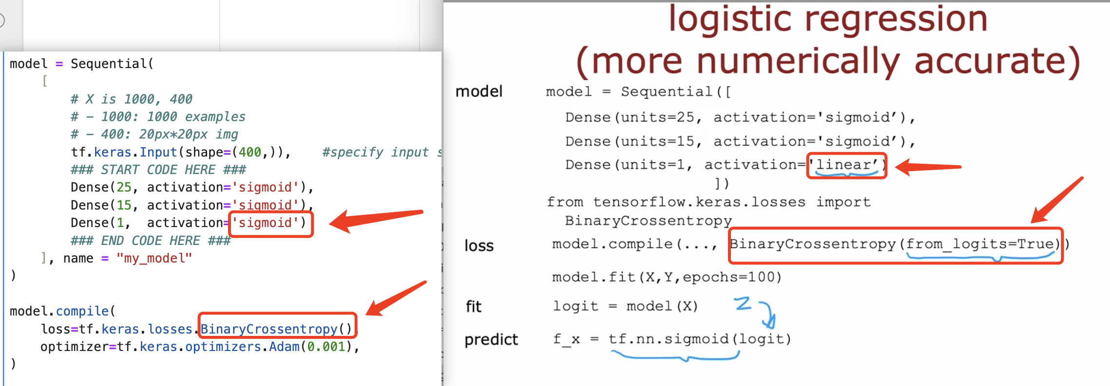
2. about softmax regression

3.7.1.6 optimization: adam

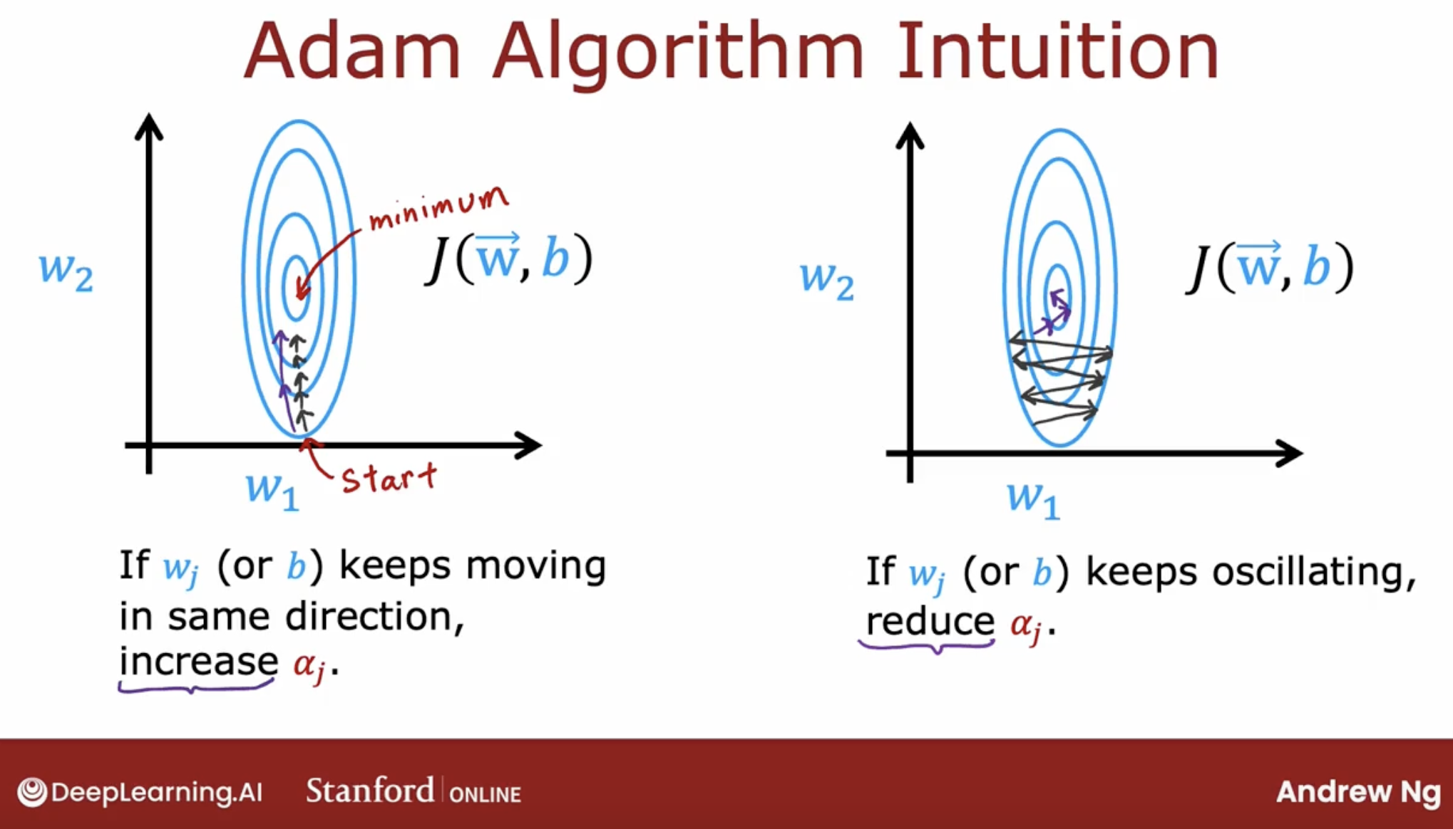
The Adam optimizer is the recommended optimizer for finding the optimal parameters of the model.

The Adam algorithm can adjust the learning rate automatically.

Adam stands for Adaptive Moment Estimation, or A-D-A-M.

The intuition behind the Adam algorithm is, if a parameter w_j, or b seems to keep on moving in roughly the same direction. This is what we saw on the first example on the previous slide. But if it seems to keep on moving in roughly the same direction, let’s increase the learning rate for that parameter. Let’s go faster in that direction.

Conversely, if a parameter keeps oscillating back and forth, this is what you saw in the second example on the previous slide. Then let’s not have it keep on oscillating or bouncing back and forth. Let’s reduce Alpha_j for that parameter a little bit.

The details of how Adam does this are a bit complicated and beyond the scope of this course, but if you take some more advanced deep learning courses later, you may learn more about the details of this Adam algorithm.

3.7.2 code

multiple_handwritten_digit_recognization

3.8 About multi labels problem

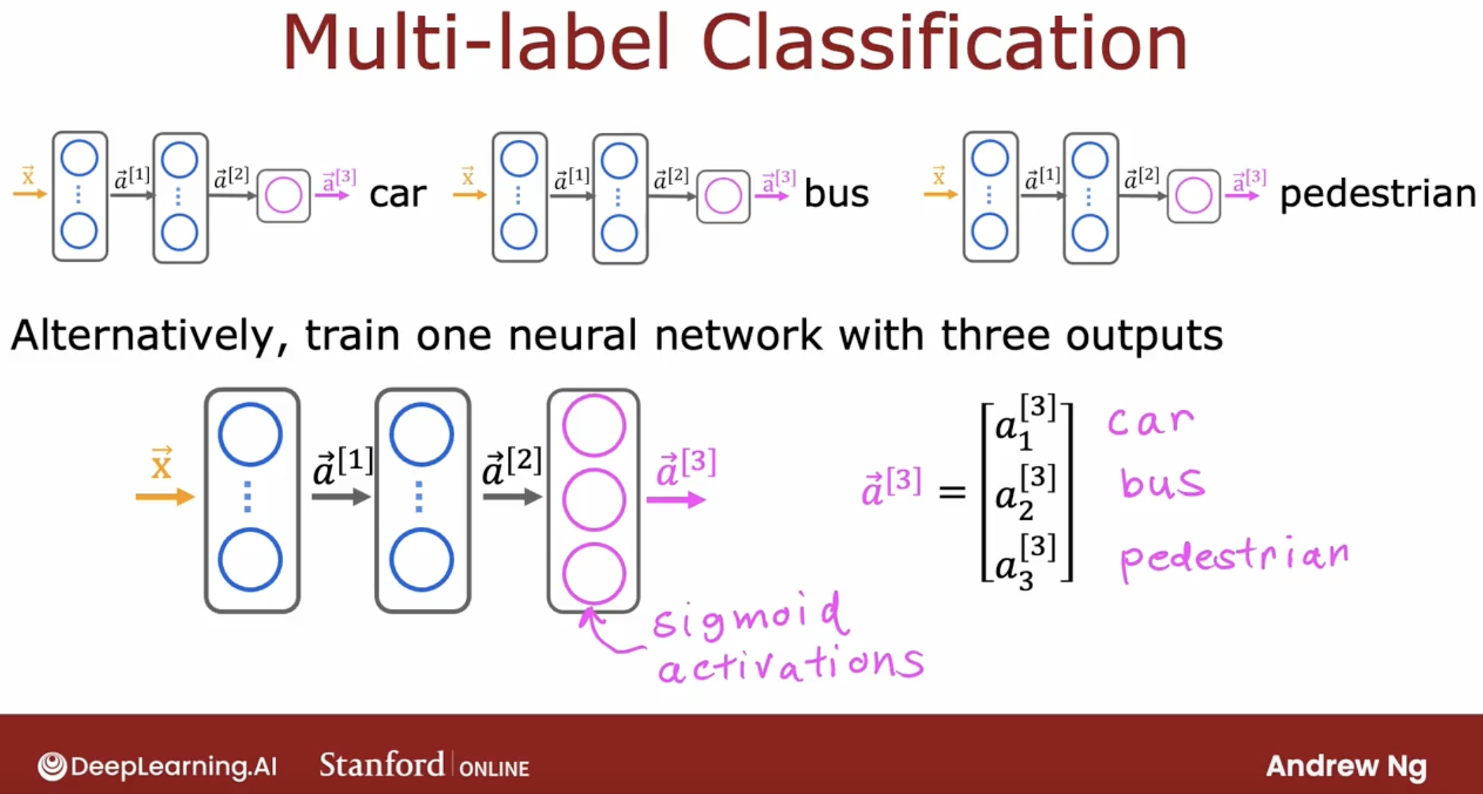
What’s multi labels problem?

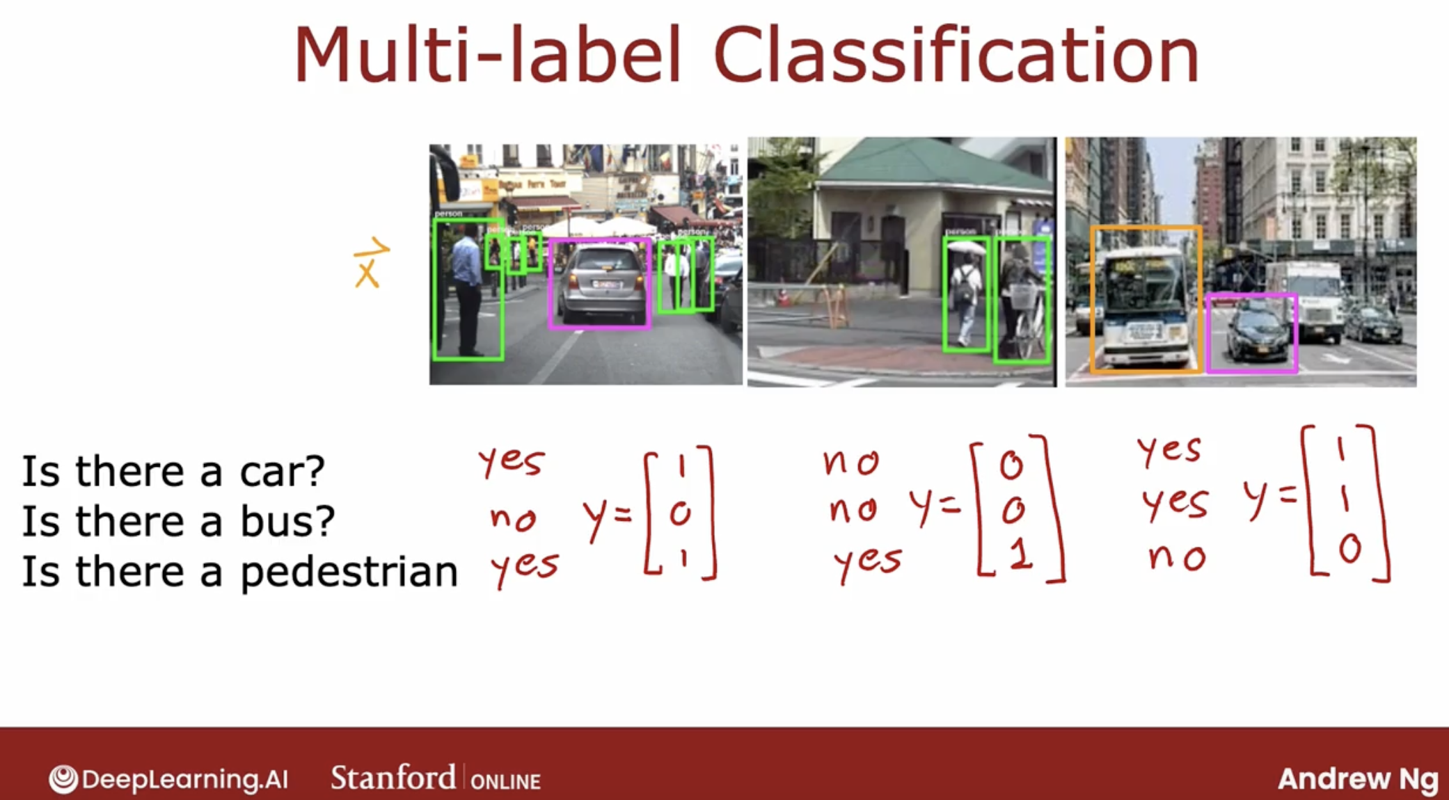
How to solve multi labels problem?

• one, surely you can train muliple neural networks, one for each label, but it’s not good.
• two, you can use the multi-label neural network.

well, we may add a demo for this situation. MARK: wait to complete.

3.9 About different layers

1. dense layer: every neuron in the layer gets its inputs all the activations from the previous layer.

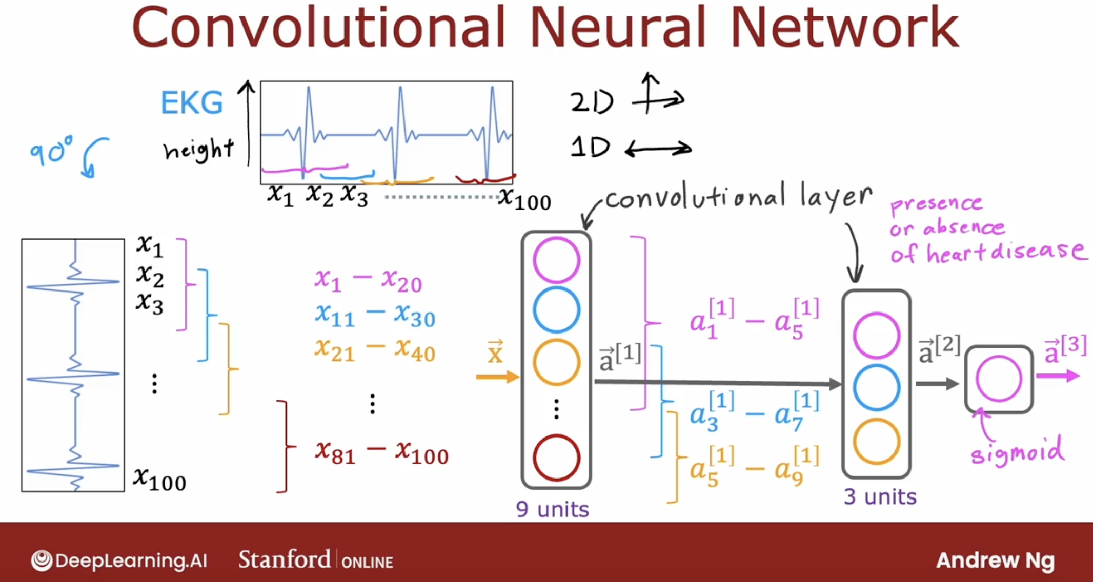
2. convolutional layer:

this is the type of layer where each neuron only looks at a region of the input image is called a convolutional layer.

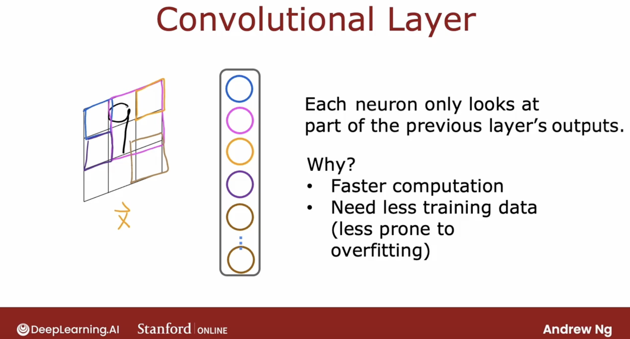
And it turns out that with convolutional layers you have many architecture choices such as how big is the window of inputs that a single neuron should look at and how many neurons should layer have.

And by choosing those architectural parameters effectively, you can build new versions of neural networks that can be even more effective than the dense layer for some applications.

1. other type layers:

And in fact, if you sometimes hear about the latest cutting edge architectures like a transformer model or an LS TM or an attention model.

A lot of this research in neural networks even today pertains to researchers trying to invent new types of layers for neural networks. And plugging these different types of layers together as building blocks to form even more complex and hopefully more powerful neural networks.

more layers