【Meachine Learning】06 Logistic Regression
1 background
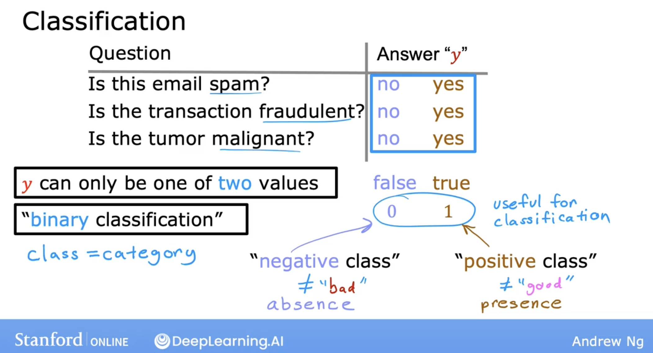
first, let’s see an example of classification problem. and is the simplest example, binary classification.
why logistic regression? why not linear regression?
because linear regression will cause miss-classification.
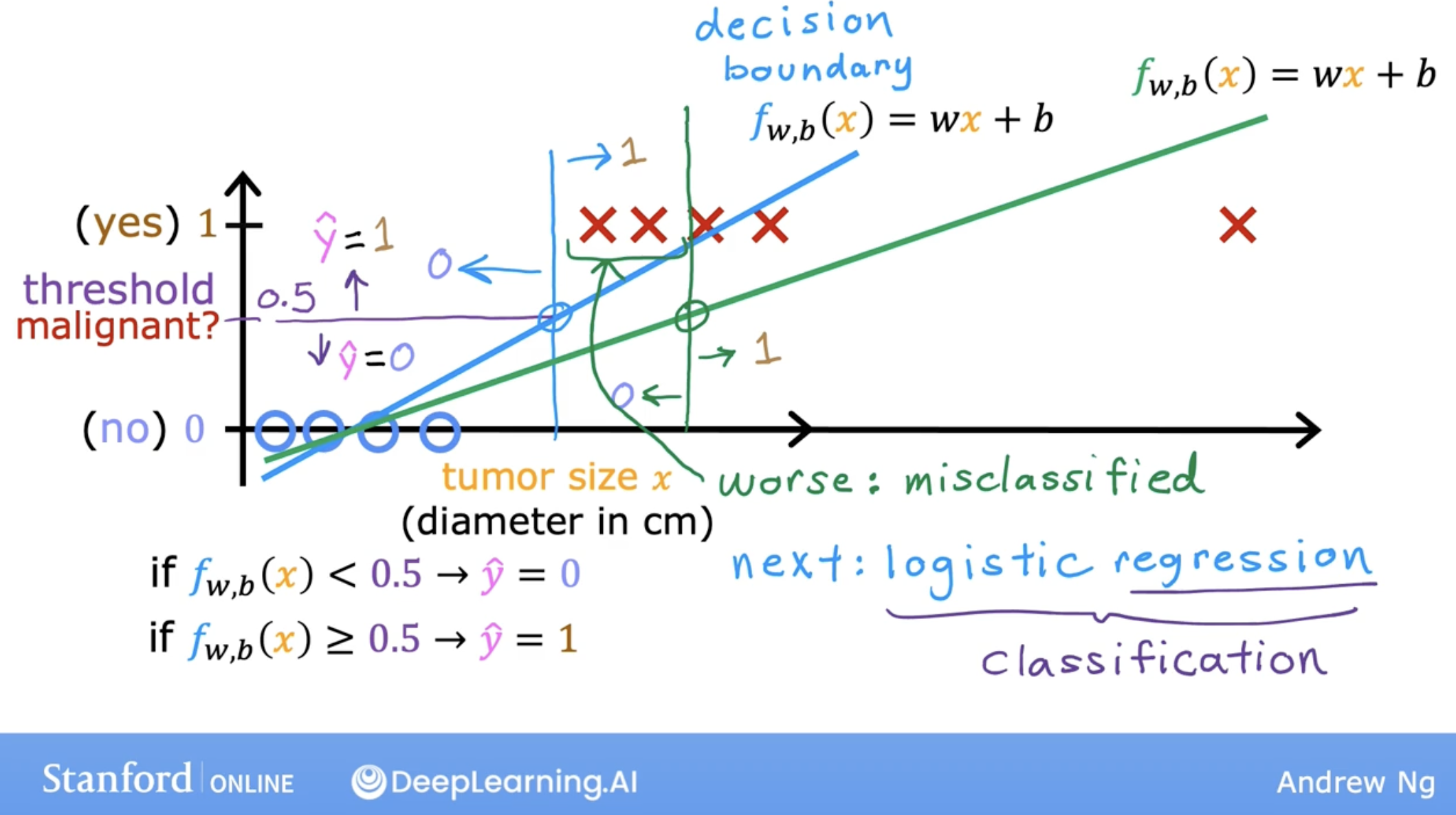
so we need to use logistic regression.
1.1 explanation
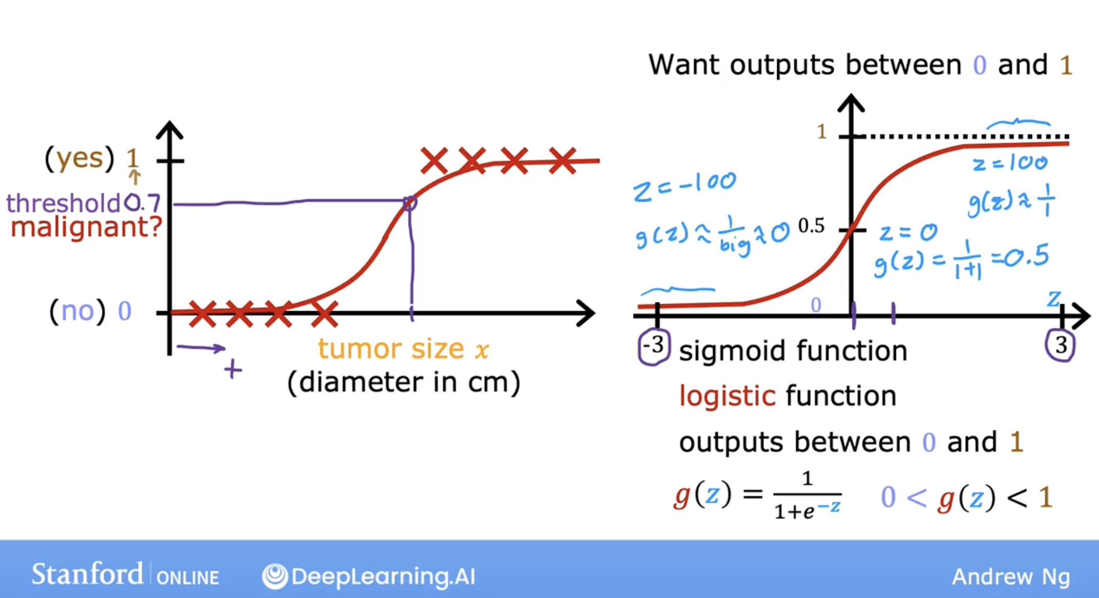
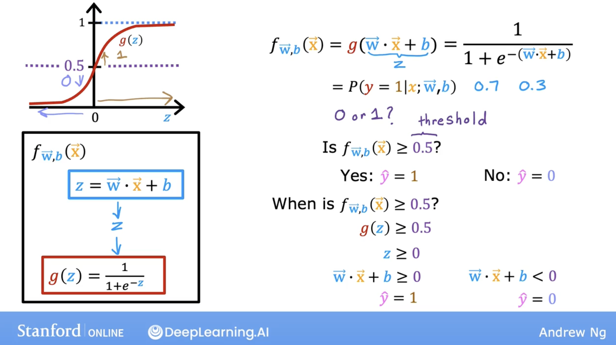
Let’s store this value in a variable which I’m going to call z, and this will turn out to be the same z as the one you saw on the previous slide.
\[z = \mathbf{w} \cdot \mathbf{x}^{(i)} + b\]and we use the following model to let output always be between 0 and 1.
\[g(z) = \frac{1}{1+e^{-z}}\]so, summary of logistic regression is:
\[f_{\mathbf{w},b}(\mathbf{x}^{(i)}) = g(\mathbf{w} \cdot \mathbf{x}^{(i)} + b ) = \frac{1}{1+e^{-(\mathbf{w} \cdot \mathbf{x}^{(i)} + b)}}\]this is also called S-shapd curve or sigmoid function or logistic function.
So we can use this function to predict the probability that y is 1 given x, and let 0.5 as the threshold, then we can get the prediction.
about threshold:
- You would not want to miss a potential tumor, so you will want a low threshold.
- A specialist will review the output of the algorithm which reduces the possibility of a ‘false positive’.
1.2 summary
To recap, what you’ve seen here is that the model predicts 1 whenever w.x plus b is greater than or equal to 0.
Conversely, when w.x plus b is less than zero, the algorithm predicts y is 0.
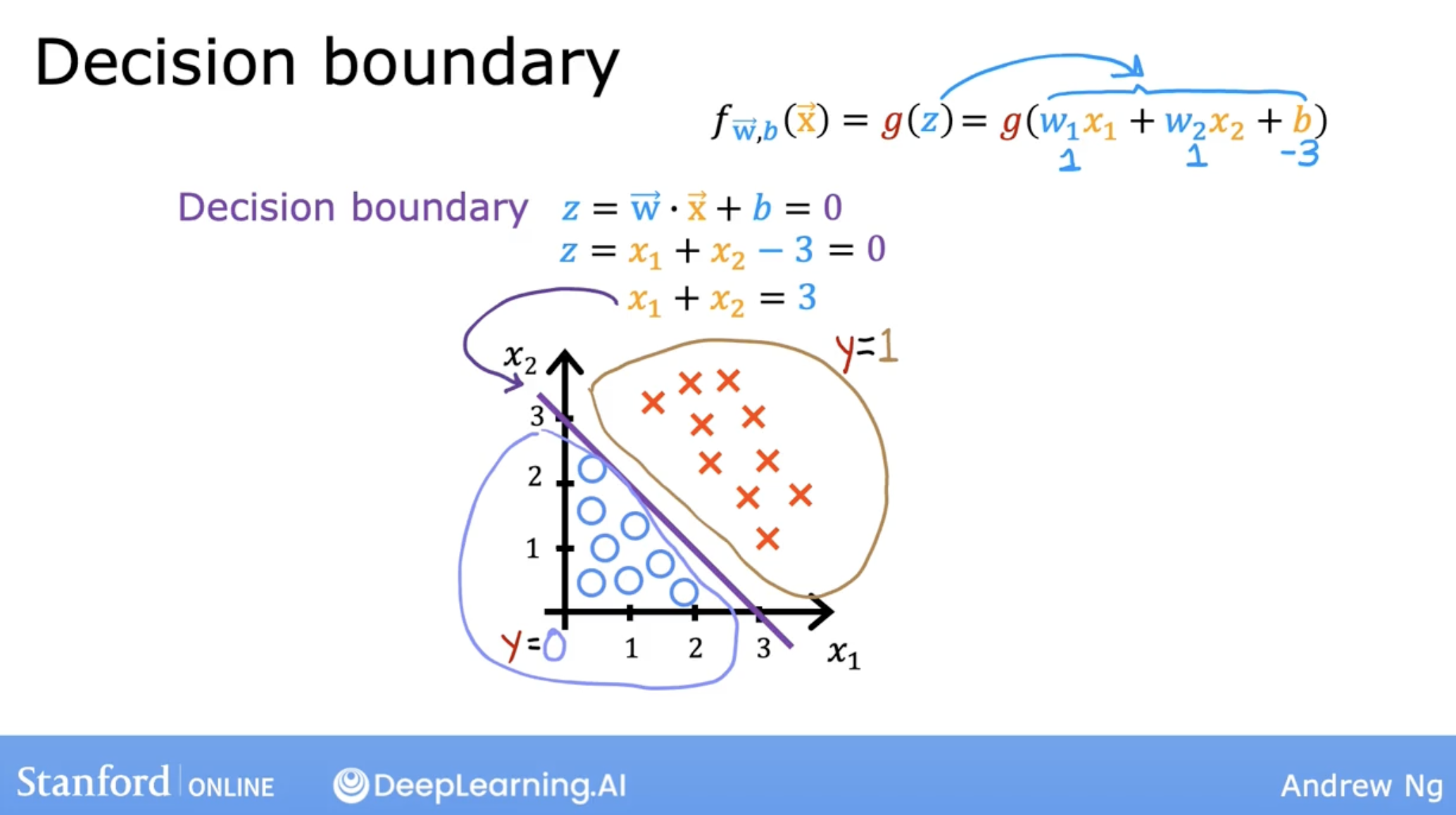
2 decision boundary
It turns out that this line is also called the decision boundary because that’s the line where you’re just almost neutral about whether y is 0 or y is 1.
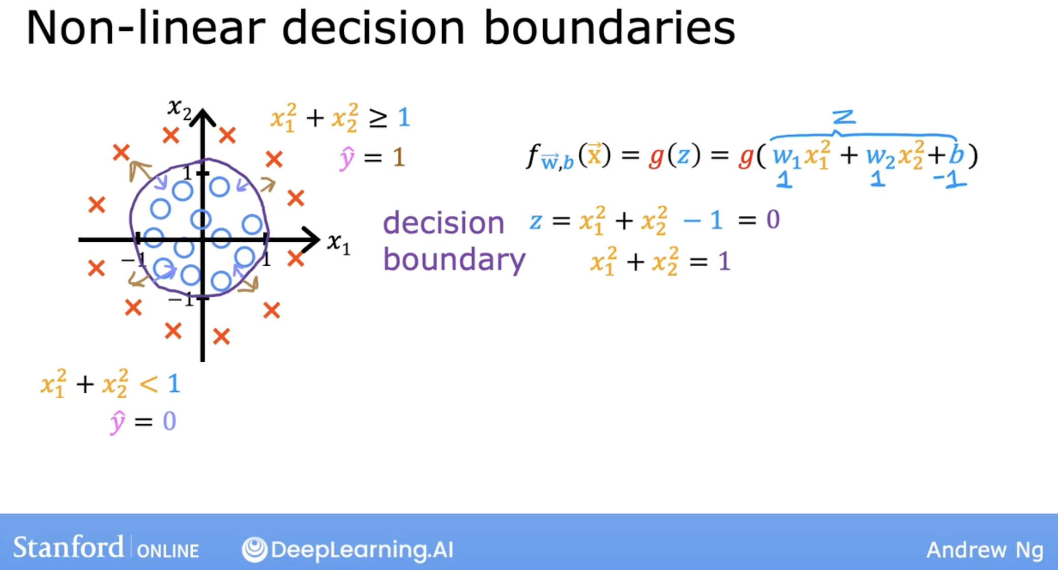
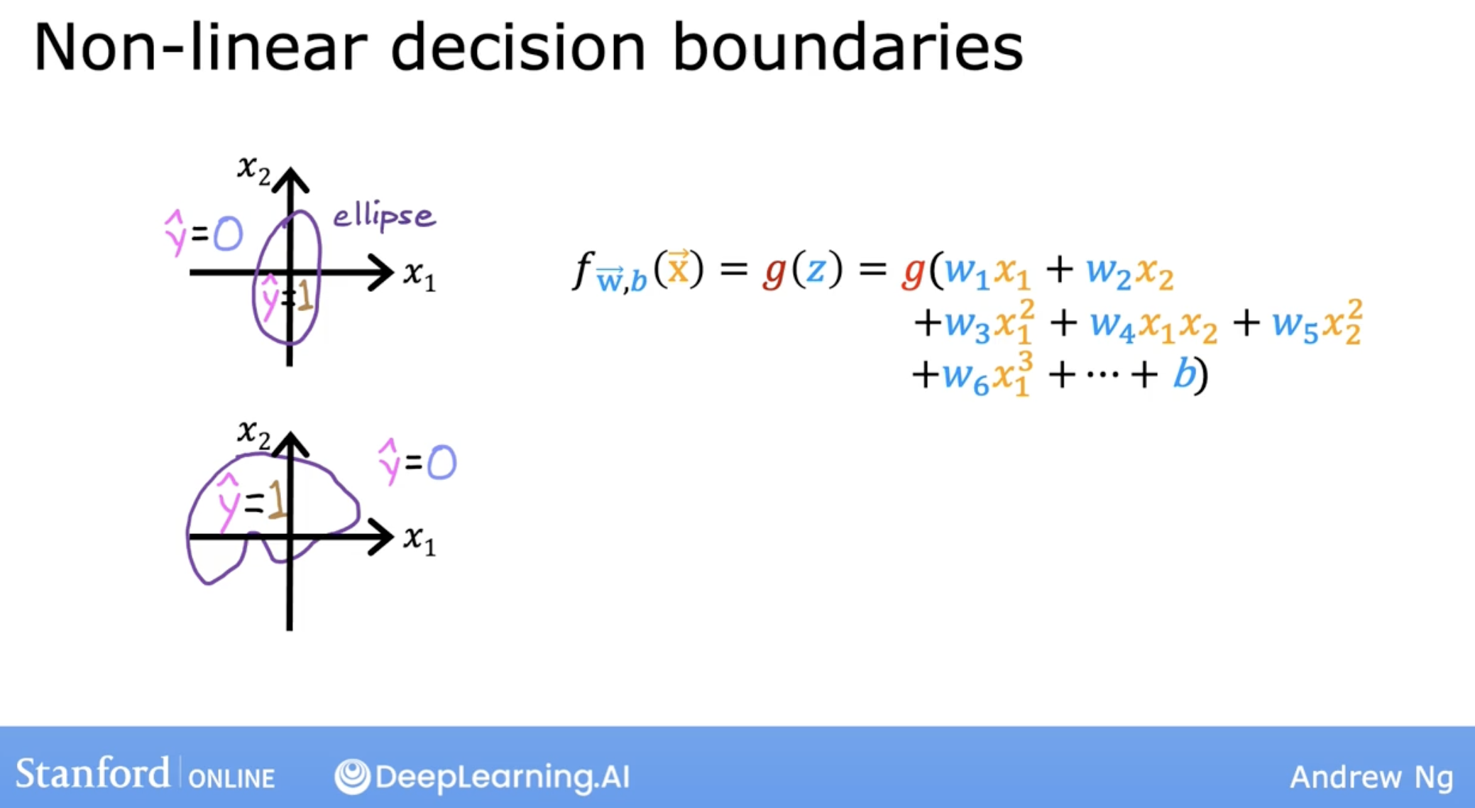
With these polynomial features, you can get very complex decision boundaries. In other words, logistic regression can learn to fit pretty complex data. even include the straight line.
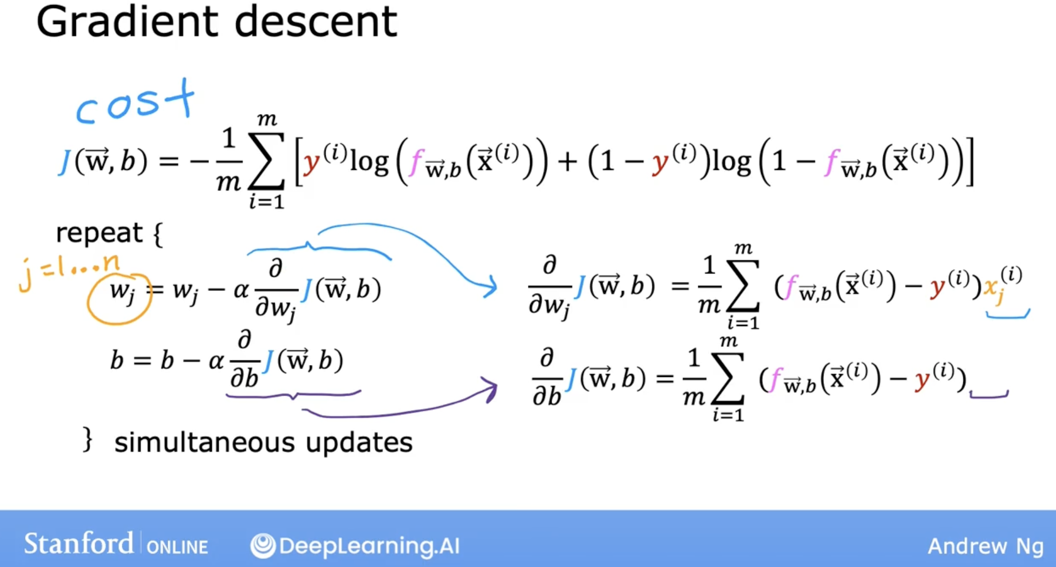
3 cost function
squared error cost function is not an ideal cost function for logistic regression.

we use the following logistic loss function
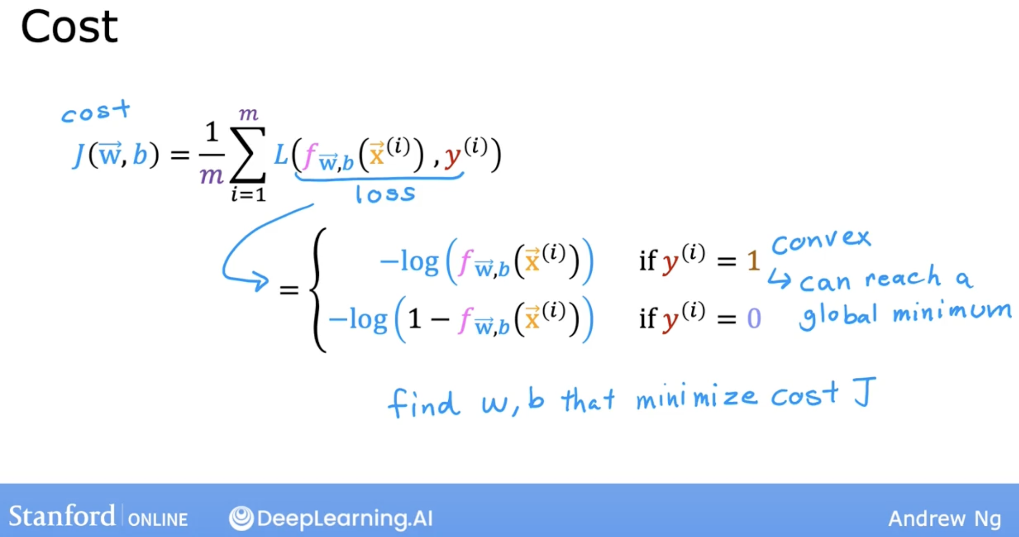
why use this logistic loss function?
- Although we won’t have time to go into great detail on this in this class, I’d just like to mention that this particular cost function is derived from statistics using a statistical principle called maximum likelihood estimation, which is an idea from statistics on how to efficiently find parameters for different models.
- This cost function has the nice property that it is convex.
- But don’t worry about learning the details of maximum likelihood.
- It’s just a deeper rationale and justification behind this particular cost function.
let’s optimize this cost function.
\[loss(f_{\mathbf{w},b}(\mathbf{x}^{(i)}), y^{(i)}) = (-y^{(i)} \log\left(f_{\mathbf{w},b}\left( \mathbf{x}^{(i)} \right) \right) - \left( 1 - y^{(i)}\right) \log \left( 1 - f_{\mathbf{w},b}\left( \mathbf{x}^{(i)} \right) \right)\] \[J(\mathbf{w},b) = \frac{1}{m} \sum_{i=0}^{m-1} \left[ -y^{(i)} \log\left(f_{\mathbf{w},b}\left( \mathbf{x}^{(i)} \right) \right) - \left( 1 - y^{(i)}\right) \log \left( 1 - f_{\mathbf{w},b}\left( \mathbf{x}^{(i)} \right) \right) \right] + \frac{\lambda}{2m} \sum_{j=0}^{n-1} w_j^2\]4 gradient descent
the gradient descent is the same as linear regression.