【Meachine Learning】02 Linear Regression with One Feature

simplest demo

intuition with simplest demo

we have a training set of data, and we want to predict the value of a target variable. how to do it?

breifly, here are the steps:

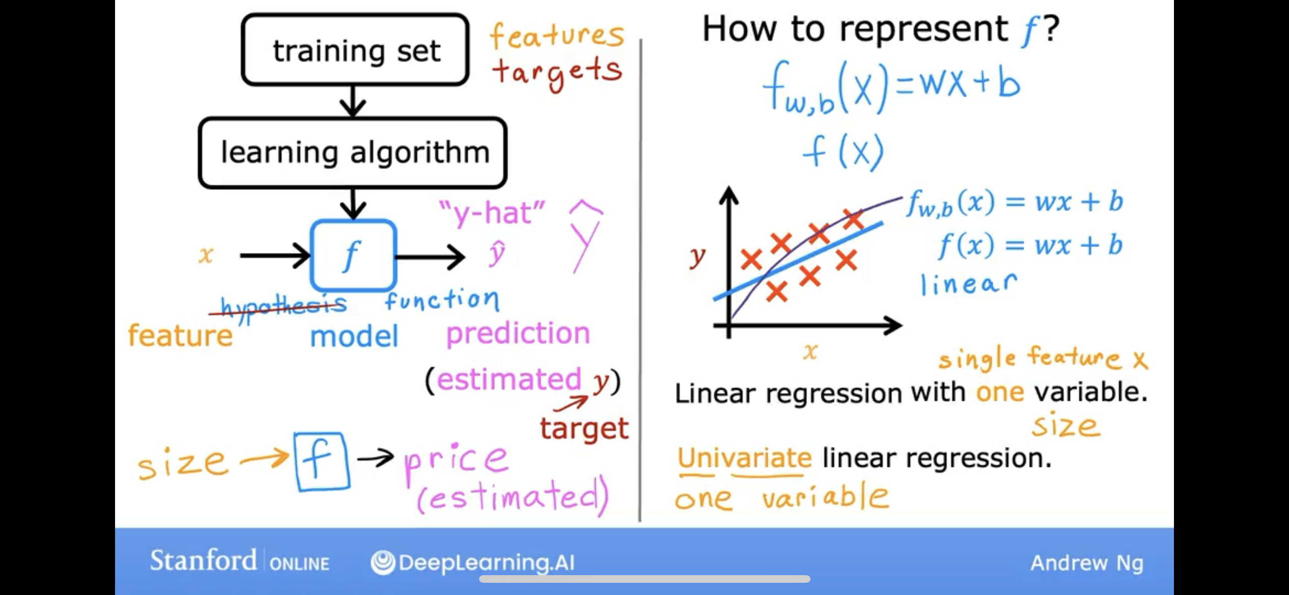
1. we have much known data, called training set;
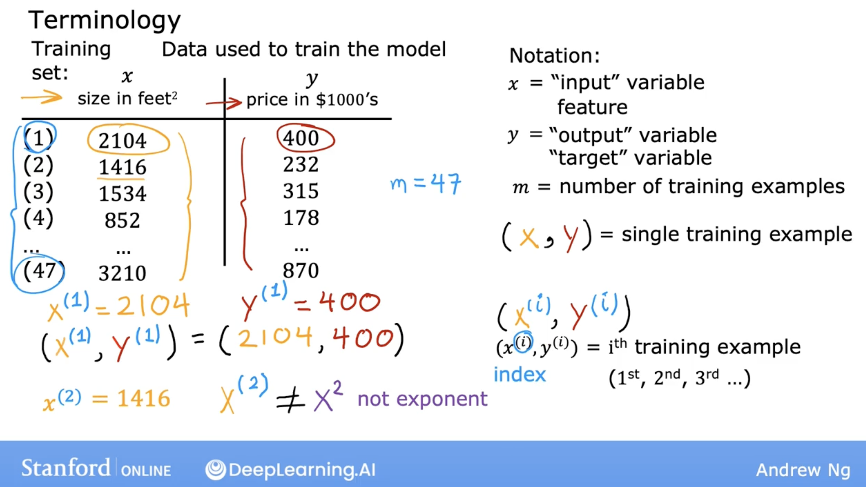
2. based on the training set, we can build a model;

\[f_{w,b}(x) = wx + b\]

1. we can use the model to predict the value of the target variable;

so, there are one question, it’s obviouls your model can not predict all the data, but how to measure the model’s performance?

we can use the cost function to measure the model’s performance.

cost function with simplest demo

cost function is what? let’s see an example:

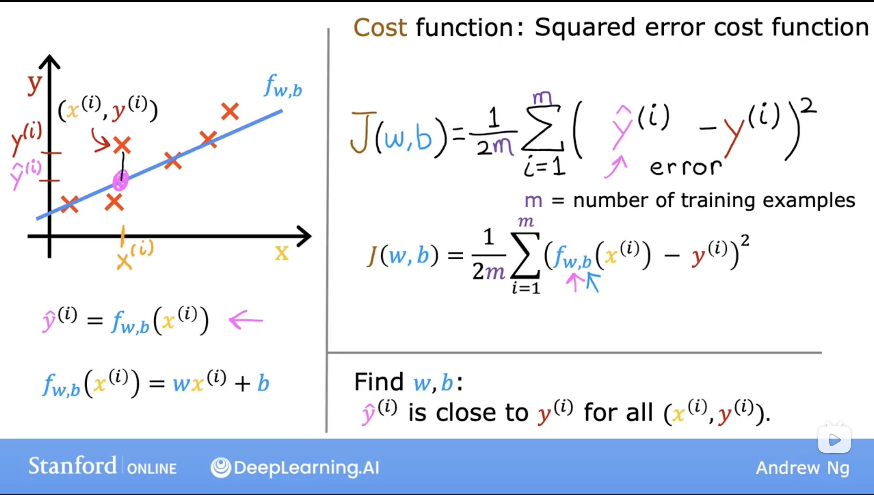
so, cost function of linear regression is \(J(w,b) = \frac{1}{2m} \sum\limits_{i = 0}^{m-1} (f_{w,b}(x^{(i)}) - y^{(i)})^2 \tag{1}\) , where \(f_{w,b}(x) = wx + b\).

we can see, the cost function is a function of two variables, \(w\) and \(b\).

in linear regression, there are surely a pair of \(w\) and \(b\), which can make this kind of cost function to be a minimum.

just like the following simple example (let’s say b = 0):

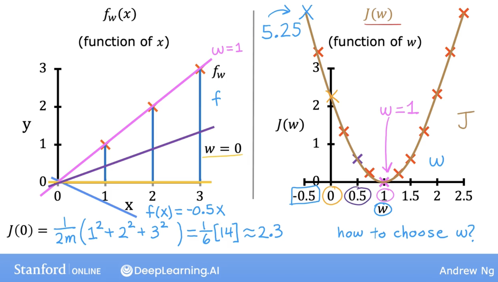
general cost function

so, what about b is not 0? J(w,b) will be a 3D function, and we can see the following example:

and even we add b, in linear regression, there are surely a pair of \(w\) and \(b\), which can make this kind of cost function to be a minimum.

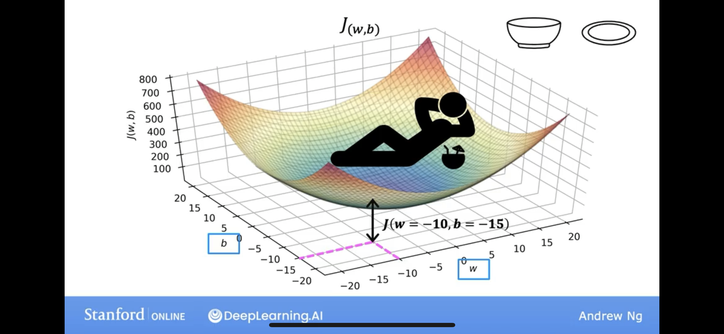
well, it’s like a bowl shape, or a hammock shape.

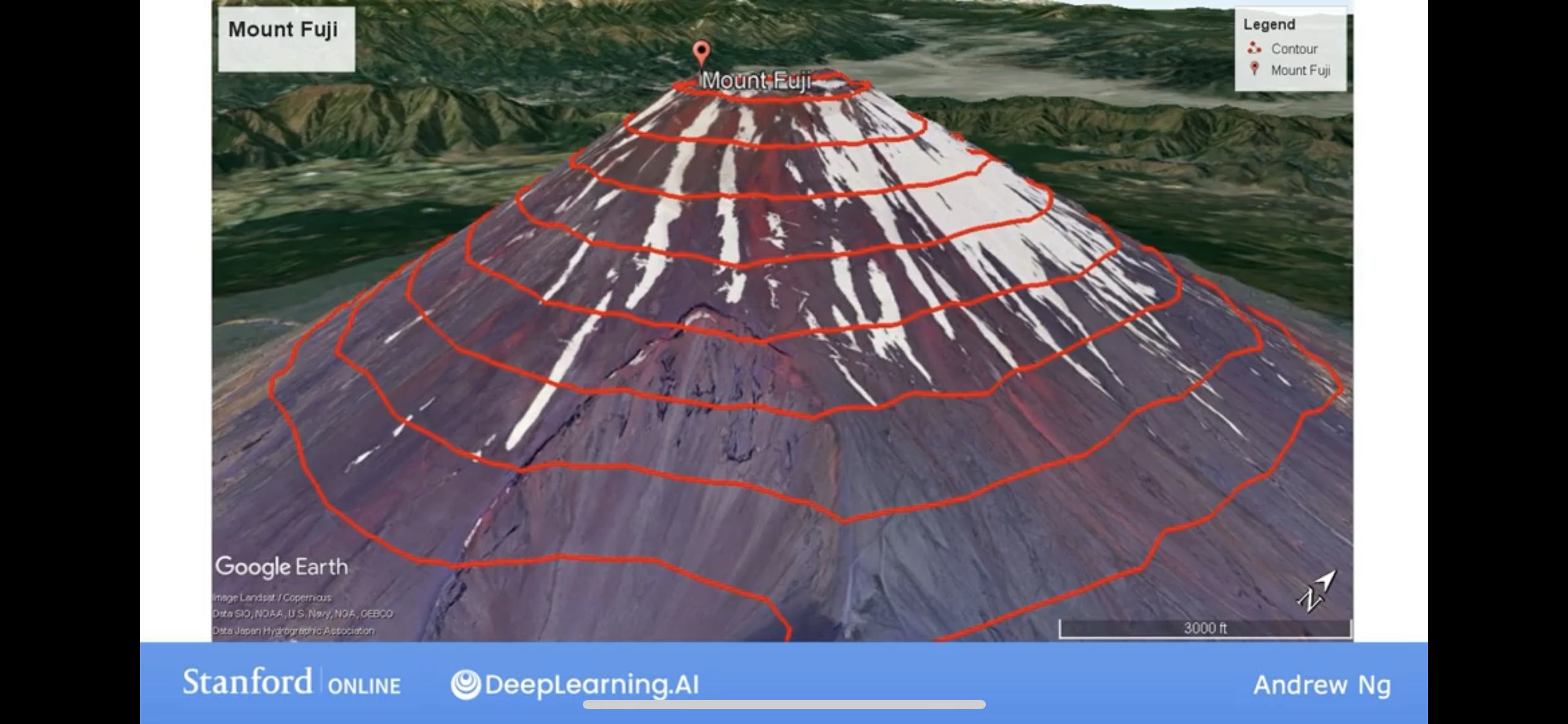
if we look this from the below, we can see, it looks like you are looking down at a mountain from the air.

Imagine we cut the mountain horizontally with a knife, we can get a contour map.

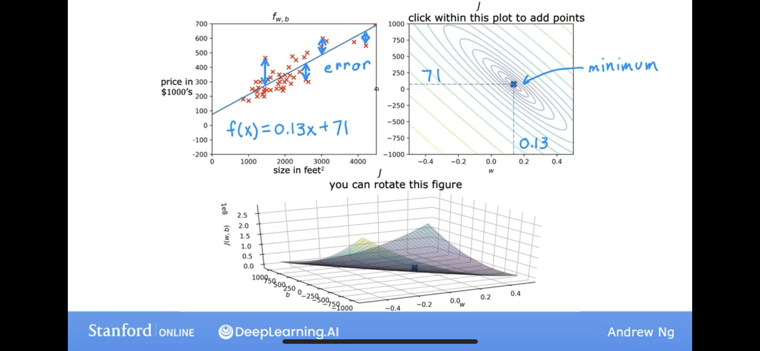
let put these three plots together:

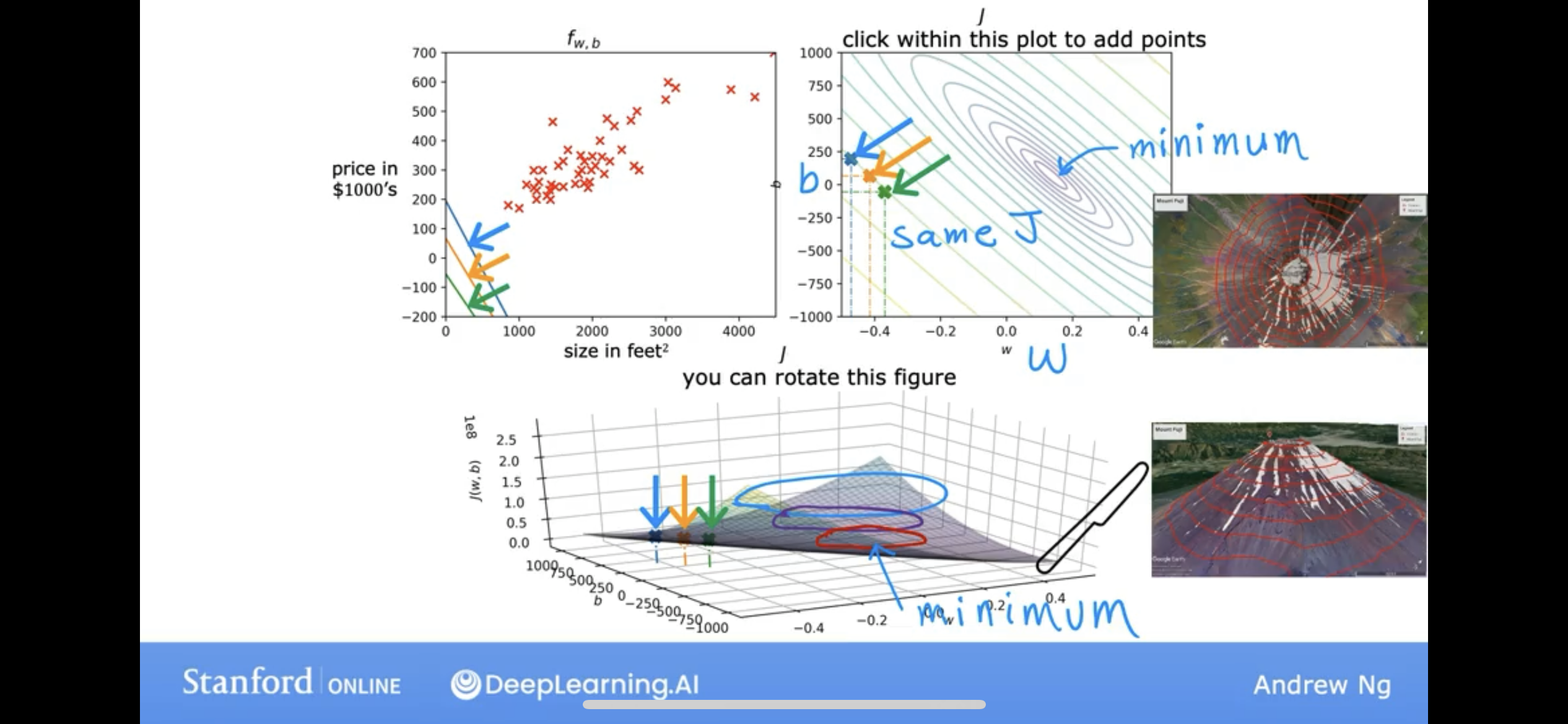
so, as the cost closer to the minimum, the model, f(x) is better.

But, there is a question, how to find the minimum? Let’s see the Gradient Descent.

Gradient Descent

general intuition

Let’s see an example to understand the Gradient Descent.

I’d like you to imagine if you will, that you are physically standing at this point on the hill. If it helps you to relax, imagine that there’s lots of really nice green grass and butterflies and flowers is a really nice hill.

Your goal is to start up here and get to the bottom of one of these valleys as efficiently as possible.

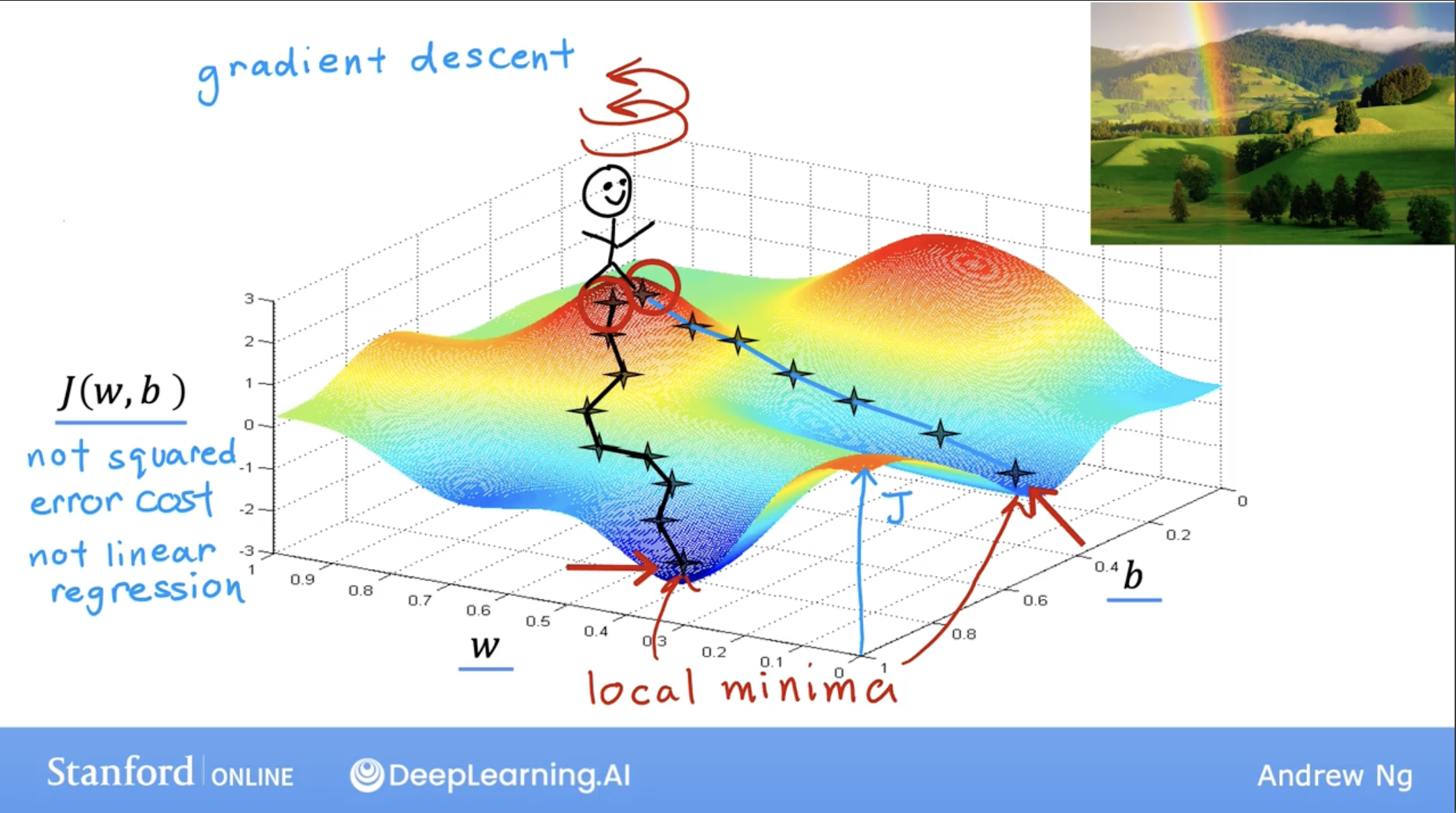
What the gradient descent algorithm does is, you’re going to spin around 360 degrees and look around and ask yourself, if I were to take a tiny little baby step in one direction, and I want to go downhill as quickly as possible to or one of these valleys. What direction do I choose to take that baby step?

Well, if you want to walk down this hill as efficiently as possible, it turns out that if you’re standing at this point in the hill and you look around, you will notice that the best direction to take your next step downhill is roughly that direction.

Mathematically, this is the direction of steepest descent.

As a reminer, you can see there may have multiple minima, the local minima. local minima: Because if you start going down the first valley, gradient descent won’t lead you to the second valley, and the same is true if you started going down the second valley, you stay in that second minimum and not find your way into the first local minima.

But don’t worry now, for linear regression with the squared error cost function, you always end up with a bowl shape or a hammock shape.

But the is a type of cost function you might get if you’re training a neural network model. we will see this in later blog.

gradient descent in linear regression

So back to our purpose, we have a cost function, and we want to find the minimum of this cost function.

so the outline is:

• Start with some w, b
• Keep changing w, b to reduce J(w, b)
• Until we settle at or near a minimum

let’s see detail step by step:

1 Start with some w, b

And in linear regression, because the squared error cost function always a bowl shape, so it won’t matter too much what the initial value are, so a common choice is to set them both to 0.

2 Keep changing w, b to reduce J(w, b)

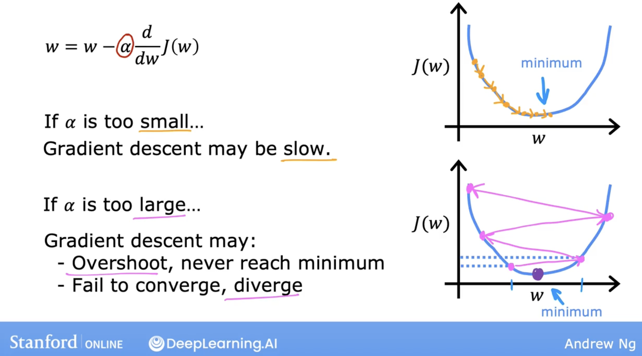
\[\begin{align*}& \text{repeat until convergence:} \; \lbrace \newline \; & \phantom {0000} b := b - \alpha \frac{\partial J(w,b)}{\partial b} \tag{1} \newline \; & \phantom {0000} w := w - \alpha \frac{\partial J(w,b)}{\partial w} \tag{2} \; & \newline & \rbrace \end{align*}\]

2.1 $\alpha$ is the learning rate.

What Alpha does is, it basically controls how big of a step you take downhill.

The learning rate is always a positive number.

If Alpha is very large, then:

• that corresponds to a very aggressive gradient descent procedure where you’re trying to take huge steps downhill.
• So if the learning rate is too large, then creating the sense may overshoot and may never reach the minimum.

If Alpha is very small, then:

• you’d be taking small baby steps downhill.
• So to summarize if the learning rate is too small, then gradient descents will work, but it will be slow. It will take a very long time because it’s going to take these tiny tiny baby steps. And it’s going to need a lot of steps before it gets anywhere close to the minimum.

2.2 partial derivative of cost function

\[\frac{\partial J(w,b)}{\partial b} = \frac{1}{m} \sum\limits_{i = 0}^{m-1} (f_{w,b}(x^{(i)}) - y^{(i)}) \tag{3}\] \[\frac{\partial J(w,b)}{\partial w} = \frac{1}{m} \sum\limits_{i = 0}^{m-1} (f_{w,b}(x^{(i)}) -y^{(i)})x^{(i)} \tag{4}\]

where:

• 3: m is the number of training examples in the dataset
• 4: $f_{w,b}(x^{(i)})$ is the model’s prediction, while $y^{(i)}$, is the target value

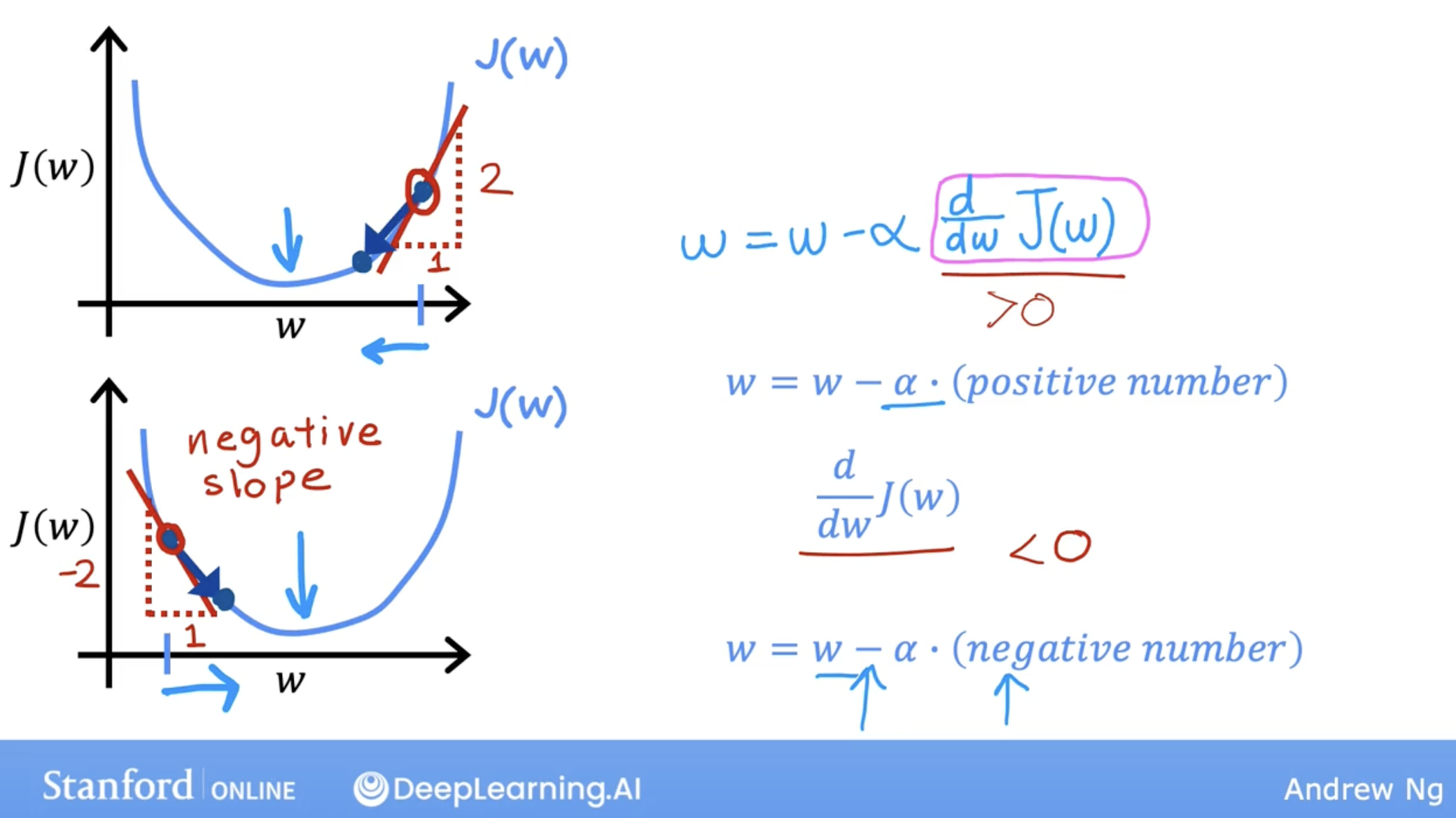
derivative: related to slope, maybe positive or negative, so w, b will be increase or decrease.

2.3 some other description

• parameters $w, b$ are both updated simultaniously and where
• Batch gradient descent:
  • And bash gradient descent is looking at the entire batch of training examples at each update.
  • To be more precise, this gradient descent process is called batch gradient descent.
  • And then it turns out that there are other versions of gradient descent that do not look at the entire training set, but instead looks at smaller subsets of the training data at each update step.
  • But we’ll use batch gradient descent for linear regression.

3 Until we settle at or near a minimum

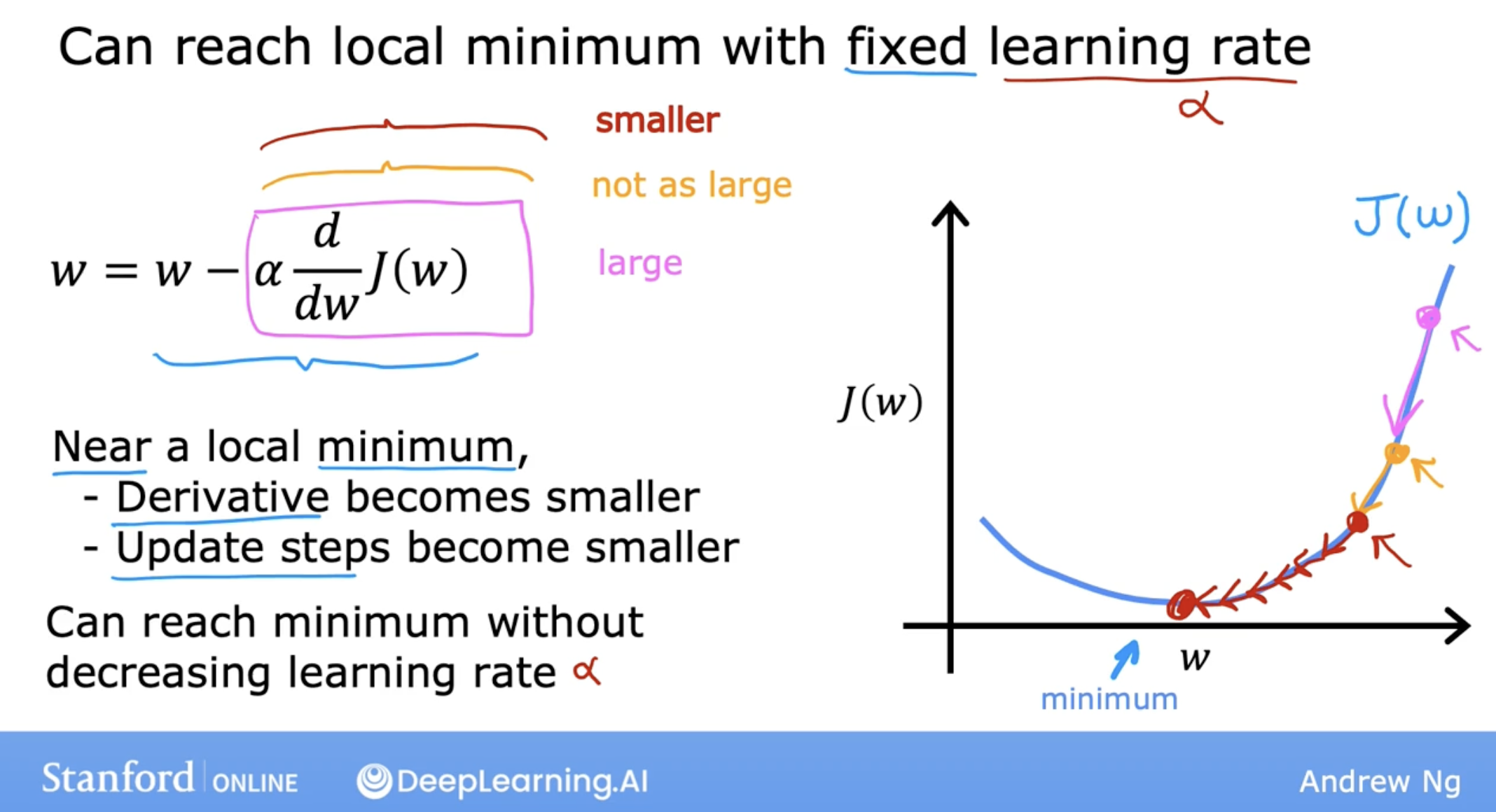
As the increase of the step, the slope of the cost function is smaller.

And you may notice that the slope is not as steep as it was at the first point. So the derivative isn’t as large. And so the next update step will not be as large as that first step.

Now, read this third point here and the derivative is smaller than it was at the previous step. And will take an even smaller step as we approach the minimum. The derivative gets closer and closer to zero.

So as we run gradient descent, eventually we’re taking very small steps until you finally reach a local minima.

So just to recap, as we get nearer a local minima gradient descent will automatically take smaller steps.

summary

model, cost function, gradient descent

Demo code

linear regression model

Wait Research Questions

some questions not answered yet, because our purpose is to use AI:

1. why cost function of linear regression is a bowl shape?
2. partial derivative vesus derivative.